ECON526: Midterm 2 Practice

Authors

Affiliation

Jesse Perla, UBC

Jesse Perla

University of British Columbia

Ungraded practice problems for Midterm 2.

Feel free to use an AI to help generate the code for the questions that depend heavily on a particular package’s API, such as the pandas tables in Question 3. Treat that as practice at prompting: describe the table you need, check that the output is what you asked for, and then write up the interpretation yourself. The interpretation is what the exam tests.

# Packages available. DO NOT MODIFY
import os
import numpy as np
import matplotlib.pyplot as plt
import scipy
import seaborn as sns
import pandas as pd
from sklearn.decomposition import PCA
from sklearn.cluster import KMeans
from numpy.linalg import cond, matrix_rank, norm
from scipy.linalg import inv, solve, det, eig, lu, eigvals
from sklearn.metrics import confusion_matrix
np.random.seed(526)

def data_path(name):
    url = "https://jlperla.github.io/grad_econ_datascience/slides/data/"
    local = f"../slides/data/{name}"
    return local if os.path.exists(local) else url + name

Short Question 1

For an \(N \times M\) matrix \(A\) with a singular value decomposition of \(A = U \Sigma V^{\top}\). Let \(u_n\) be the \(n\)-th column of \(U\), \(v_n\) be the \(n\)-th column of \(V\),

What are the dimensions of each of the terms \(U\), \(\Sigma\), and \(V\)? What are the properties or structure of each?
Use those terms to provide an interpretation for the function \(f(x) = A x = U \Sigma V^{\top} x\) for a vector \(x\).
Write \(A\) as a sum of rank 1 matrices in terms of the elements of \(\Sigma\) and the columns of \(U\) and \(V\).

Answer:

(double click to edit your answer)

Short Question 2

For an \(N \times M\) data matrix \(X\) with \(N > M\), where each column is normalized to have a mean of \(0\), with a singular value decomposition of \(X = U \Sigma V^{\top}\).

If the matrix is full rank, how many singular values are non-zero?
If we say that the first two singular values were vastly larger than the rest, explain how PCA would help us better understand the data.
What if the first two singular values were non-zero but the rest of them were zero?

Answer:

(double click to edit your answer)

Short Question 3

A classifier for whether a firm goes bankrupt within a year (\(y = 1\)) is evaluated on \(1000\) held-out firms, \(50\) of which went bankrupt. It flags \(40\) firms, \(30\) of which went bankrupt. Use the layout from the lecture:

	predicted \(\hat{y} = 0\)	predicted \(\hat{y} = 1\)
true \(y = 0\)	true negative (\(TN\))	false positive (\(FP\))
true \(y = 1\)	false negative (\(FN\))	true positive (\(TP\))

Fill in the four cells and compute the accuracy, precision, and recall.
What is the accuracy of a rule that predicts “no bankruptcy” for every firm? What does that say about using accuracy here?
The classifier works from a fitted probability \(\hat{p}(x)\) and a threshold \(\tau = 1/2\). If a missed bankruptcy costs a lender nine times as much as a false alarm, which direction should \(\tau\) move, roughly where, and what happens to precision and recall when you switch to it?

Answer:

(double click to edit your answer)

Short Question 4

Two classifiers for the same rare outcome are compared with ROC curves on held-out data, sketched below without numbers. Model A has the higher area under the curve. Model B’s curve lies above Model A’s only at the far left, at very low false positive rates.

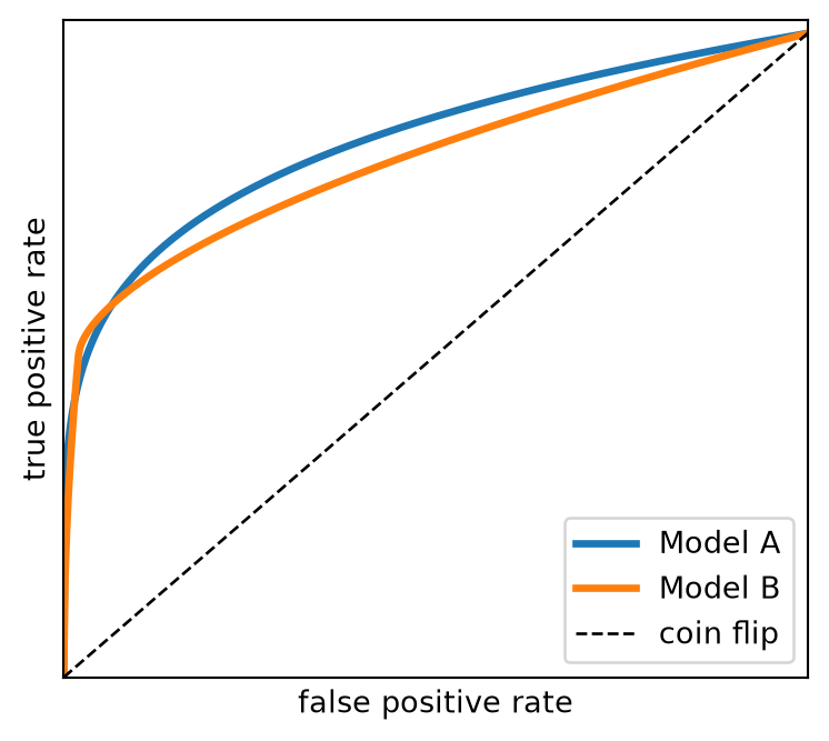
What do the axes of an ROC curve measure, and what does moving along one curve correspond to?
In what sense is Model A better, and when would you still prefer Model B?
Why does the ROC curve not change when you change the threshold, while precision and recall do?

Answer:

(double click to edit your answer)

Short Question 5

Consider the k-means objective for a partition \(\mathbf{S} = \{S_1, \ldots, S_K\}\) of observations \(x_1, \ldots, x_N \in {\mathbb{R}}^M\),

\[ \min_{\mathbf{S}} \sum_{k=1}^K \sum_{n \in S_k} \|x_n - \bar{x}_k\|_2^2 \]

Does KMeans always return the same partition when you run it twice on the same data? Why or why not, and what does n_init do about it?
Two features are measured in dollars and in millions of dollars respectively. What does the objective effectively minimize, and what should you do first?
Explain why the minimized objective is weakly decreasing in \(K\) and reaches \(0\) at \(K = N\), and what the elbow method does about that.

Answer:

(double click to edit your answer)

Short Question 6

A researcher hand-labels a random sample of \(2000\) newspaper articles for whether they cover a strike, trains a classifier on word counts, and uses it to label the other \(500{,}000\) articles.

What does TF-IDF (term frequency, inverse document frequency) change relative to raw word counts, and why might that help?
With \(6\%\) positives the default logistic fit had precision \(0.95\) and recall \(0.35\). What does class_weight="balanced" do to the fit, and what happens to the two numbers?
The predicted labels are then the outcome in a linear regression (with an intercept) of strike coverage on a regional indicator. If the classifier’s false positive and false negative rates \(p_0\) and \(p_1\) are the same in every region, with \(p_0 + p_1 < 1\), what happens to the regression coefficient, and what is the fix? Why does the fix fail if the error rates differ by region?

Answer:

(double click to edit your answer)

Short Question 7

Consider a language model with a vocabulary of \(K\) tokens.

What is the difference between a word and a token, and why do Hello world and hello world tokenize differently?
An embedding maps a token or a document to \(z = \phi(x) \in {\mathbb{R}}^L\). Why is cosine similarity \(z \cdot z' / (\|z\| \|z'\|)\) used to compare embeddings rather than \(\|z - z'\|\), and what do values of \(1\), \(0\), and \(-1\) mean?

Answer:

(double click to edit your answer)

Short Question 8

The NLP lecture described embeddings as a map \(\phi\) from some \(x \in {\mathcal{X}}\) to a latent space \({\mathcal{Z}}\).

In what sense is PCA with \(L\) components an embedding? Write the map and say what it is chosen to preserve.
How does a text embedding from a language model differ from it?

Answer:

(double click to edit your answer)

Short Question 9

A language model takes a sequence of tokens \(x_1, \ldots, x_{t-1}\) and produces a probability for each of the \(K\) possible next tokens \(x_t\).

Describe, in general terms, the steps from the token sequence to that probability distribution: what gets embedded, what the embeddings are combined into, and what the last step has to deliver.
The last step maps a latent \(z \in {\mathbb{R}}^L\) to probabilities over \(K\) outcomes. Which function from the classification lecture does that, and write it out.
You ask the same question twice, once with two words in the prompt swapped, and the model answers differently. What does that tell you about how the embedding of the sequence is built? Contrast with a bag of words.

Answer:

(double click to edit your answer)

Short Question 10

In the NLP lecture, sentence embeddings from a language model gave

\(\mathrm{sim}(e_2, e_3)\) high for “The dog chased the man” and “The man was chased by the dog”,
but \(\mathrm{sim}(e_3, e_4) > \mathrm{sim}(e_3, e_2)\) for “The man was chased by the dog” and “The man chased the dog”.

A bag-of-words embedding of a sentence is the vector of its word counts. What does it throw away, and how would it score the three sentences above relative to each other?
The second finding says that “The man was chased by the dog” is closer to “The man chased the dog”, the opposite event, than to “The dog chased the man”, the same event. Why does that mean a high cosine similarity cannot simply be read as “the same meaning”? What would you need to know to interpret it?
The local LLM lecture embedded the same words with OpenAI’s \(3072\)-dimensional model and a local \(1024\)-dimensional model. Why are the cosine values from the two models not comparable, and what comparison across them is still meaningful?
You have \(400\) hand-labelled articles and want to classify \(500{,}000\). Give one reason to prefer embeddings plus logistic regression over TF-IDF plus logistic regression in that situation, and one reason to prefer TF-IDF.

Answer:

(double click to edit your answer)

Short Question 11

The local LLM lecture ran open-weight models through Ollama with the same openai Python client as the hosted models.

What does “open-weight” mean, and what changes when you run such a model on your own machine rather than calling a hosted API?

Answer:

(double click to edit your answer)

Short Question 12

What are the tradeoffs of using a local open-weight model rather than a hosted frontier model such as OpenAI’s for a research task, say classifying a few hundred thousand documents?

Answer:

(double click to edit your answer)

Question 1

Take the following model from our problem set, and modify it so that the generated data has circles which overlap so the data isn’t fully separated. You should consider overlapping symmetrically vs. asymmetrically.

# MODIFY CODE HERE
def generate_noisy_circle(radius, num_points, noise_std):
    theta = np.linspace(0, 2*np.pi, num_points)
    x = radius * np.cos(theta) + np.random.normal(0, noise_std, num_points)
    y = radius * np.sin(theta) + np.random.normal(0, noise_std, num_points)
    return np.column_stack((x, y))

# Generate data for inner and outer circles
X_1 = generate_noisy_circle(0.5, 100, 0.05)
X_2 = generate_noisy_circle(1.5, 100, 0.05)

# Create dataframes
df_1 = pd.DataFrame({"f1": X_1[:, 0], "f2": X_1[:, 1], "k": 0})
df_2 = pd.DataFrame({"f1": X_2[:, 0], "f2": X_2[:, 1], "k": 1})
df = pd.concat([df_1, df_2], ignore_index=True)
fig, ax = plt.subplots(figsize=(6, 4))
sns.scatterplot(data=df, x="f1", y="f2", hue="k", ax=ax)
ax.set(xlabel="Feature 1", ylabel="Feature 2", title="Latent Groups")
plt.show()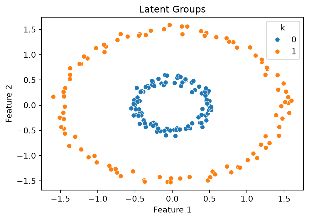

Given the above code, the following should provide the confusion matrix without modification

# DO NOT MODIFY
kmeans = KMeans(n_clusters=2, random_state=0)
df["k_hat"] = kmeans.fit_predict(df[["f1", "f2"]])

# Create confusion matrix
cm = confusion_matrix(df["k"], df["k_hat"])

# Plot confusion matrix
sns.heatmap(cm, annot=True, cmap='Blues')
plt.xlabel('Predicted k')
plt.ylabel('True k')
plt.title('Confusion Matrix for K-Means Clustering')
plt.show()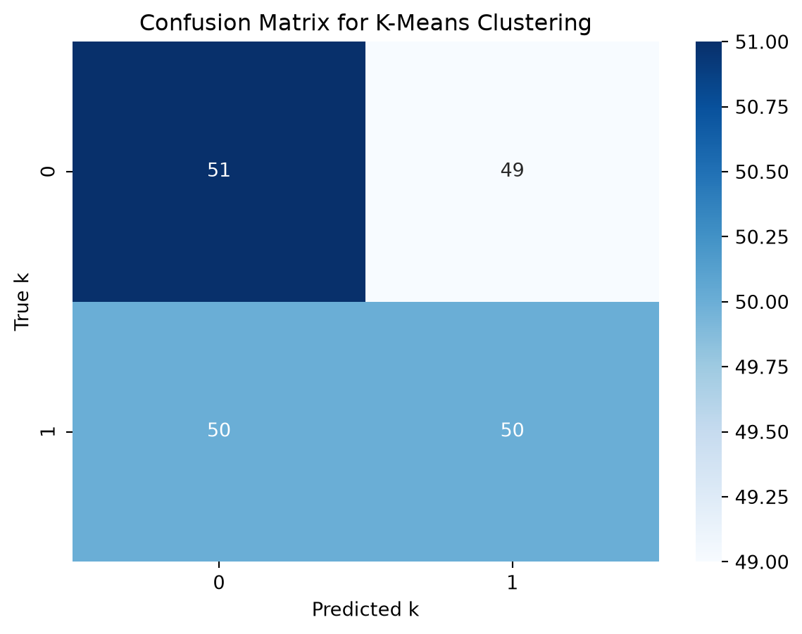

Did the performance of the k-means clustering get better, worse, or the same? Briefly explain, referring to math if possible

Answer:

(double click to add an explanation here)

Question 2

The features in X below have similar variances and PCA recovers a first direction that loads on all three.

N = 50
Z = np.random.randn(N, 2)
F = np.array([[1.0, 0.05], [2.0, 0.0], [3.0, 0.1]])
X = Z @ F.T + 0.1 * np.random.randn(N, 3)
pca_X = PCA(n_components=3).fit(X)
print(f"first principal direction: {pca_X.components_[0].round(3)}")

first principal direction: [0.268 0.527 0.806]

Question 2.1

Multiply the first feature by \(100\), as if it switched from dollars to cents, and refit. Report the first principal direction and the explained variance ratios. What happened and why?

# modify here

Answer:

(double click to edit your answer)

Question 2.2

Standardize each column of the rescaled data (subtract its mean and divide by its standard deviation) and refit. Compare the first direction to the two previous ones and explain which analysis you would trust.

# modify here

Answer:

(double click to edit your answer)

Question 3

The image classification lecture asked several models to label \(100\) satellite chips with one of ten land-use classes: four open-weight vision models each once zero-shot (examples = 0) and once with ten example chips in the prompt (examples = 10), gpt-4o-mini zero-shot only, and a Vision Transformer fine-tuned on \(21{,}600\) labelled chips (examples = 0 for that row means no prompt examples, not no training). The predictions are stored, so nothing here needs a model.

preds = pd.read_csv(data_path("eurosat_predictions.csv"), keep_default_na=False)
preds["correct"] = preds["predicted"] == preds["truth"]
print(preds.head())

   index        truth       model  examples         answer      predicted  \
0      0      SeaLake  qwen3.5:2b         0  PermanentCrop  PermanentCrop   
1      1  Residential  qwen3.5:2b         0     Industrial     Industrial   
2      2  Residential  qwen3.5:2b         0  PermanentCrop  PermanentCrop   
3      3      SeaLake  qwen3.5:2b         0  PermanentCrop  PermanentCrop   
4      4   Industrial  qwen3.5:2b         0     Industrial     Industrial   

   correct  
0    False  
1    False  
2    False  
3    False  
4     True

Question 3.1

Compute the accuracy of each model with and without examples, as one table with a row per model. Which model is best, and what do the examples buy?

Hint: unless you already know pivot_table, use this as practice in asking an AI for help with the code that produces the table, check that the table is what you asked for, then write the analysis in your own words.

# modify here

Answer:

(double click to edit your answer)

Question 3.2

Take gpt-4o-mini zero-shot. Cross-tabulate the true class against the predicted class, then compute precision and recall for the SeaLake class and for the Residential class. With ten classes, what are the “positives” and “negatives” in those definitions, and which other classes does the model confuse with each?

Hint: as in Question 3.1, the code is the kind of thing to ask an AI for. A prompt that works spells out the table and the counts you need, for example:

I have a pandas DataFrame called preds with the columns truth, predicted, model, and examples. Please write Python that (1) keeps only the rows where model is "gpt-4o-mini" and examples is 0, (2) prints a cross-tabulation of truth (rows) against predicted (columns), and (3) for each of the classes "SeaLake" and "Residential", treating that class as the positive class and every other class as negative, computes the true positives, false positives, and false negatives and prints precision and recall.

The interpretation that follows is yours to write.

# modify here

Answer:

(double click to edit your answer)

Reuse

CC BY-NC-SA 4.0

Other Formats

Short Question 1

Answer:

Short Question 2

Answer:

Short Question 3

Answer:

Short Question 4

Answer:

Short Question 5

Answer:

Short Question 6

Answer:

Short Question 7

Answer:

Short Question 8

Answer:

Short Question 9

Answer:

Short Question 10

Answer:

Short Question 11

Answer:

Short Question 12

Answer:

Question 1

Answer:

Question 2

Question 2.1

Answer:

Question 2.2

Answer:

Question 3

Question 3.1

Answer:

Question 3.2

Answer:

Reuse