Stochastic Asset Pricing and Expected Present Discounted Values
Honours Intermediate Macro
Asset pricing with Markov chains, linear state space models with uncertainty, and stochastic bubbles
Asset Pricing with Markov Chains
Stochastic Asset Pricing with Discrete States
Setup:
- Assume a discrete number, \(1,\ldots N\), of possible states of the world
- Let \(P\) be the transition matrix of the Markov chain for these states, and let \(A \equiv P^\top\) (the transpose)
- If \(\pi_t\) is the pmf as a row vector, let \(x_t \equiv \pi_t^\top\) be the distribution (pmf) of possible states for the random variable as a column vector
Take the standard forecast, \(\pi_{t+1} = \pi_t P\) and take the transpose of both sides to get \(x_{t+1} \equiv \pi_{t+1}^\top = (P^\top \pi_t^\top) = A x_t\). Then we see the forecast \(j\) into the future is
\[ x_{t+j} = A^j \cdot x_t \]
Let the payoff in each state be \(G=\begin{bmatrix}y_1 & \cdots & y_N \end{bmatrix}\), so
\[ y_t = \begin{bmatrix}y_1&\cdots &y_N\end{bmatrix} \cdot \begin{bmatrix}x_{1t}\\x_{2t}\\ \vdots \\ x_{nt}\end{bmatrix} = G\cdot x_t \]
Given the possible payout states, the random variable \(Y_t\) is all of the possible payouts in \(G\) with probability \(x_t\). So
\[ y_t \equiv {\mathbb{E}_{{t}}\left[ {Y_t} \right]} = G x_t \]
Compare to the linear state space model: \(x_{t+1} = A x_t\) and \(y_t = G x_t\).
Example:
- \(y_t = y_1\) if \(x_{1t} = 1\)
- \(y_t = y_N\) if \(x_{Nt} = 1\)
- If 50% chance in each of the first 2 states:
\[ y_t = G \cdot x_t = \begin{bmatrix}y_1&\cdots &y_N\end{bmatrix} \cdot \begin{bmatrix}\frac{1}{2}\\\frac{1}{2}\\0 \\ \vdots \\ 0\end{bmatrix} = \frac{1}{2}y_1+\frac{1}{2}y_2 \]
This gives the expected dividends.
Using Markov chains for forecasting:
- \(x_{t+j} = A^j x_t\)
- \(y_t = G \cdot x_t\)
- Using the forecast and weighting by the pmf: \(y_{t+j} = {\mathbb{E}_{{t}}\left[ {Y_{t+j}} \right]} = G x_{t+j}\)
Asset pricing formula:
\[ p_t(x_t) = {\mathbb{E}_{{t}}\left[ {\sum_{j=0}^{\infty} \beta^j Y_{t+j}} \right]} = G\left( \sum_{j=0}^{\infty} \beta^j A^j \right)x_t \]
This is close to our old form (note that we have the transpose \(A \equiv P^\top\)):
\[ \boxed{p(x_t) = G(I-\beta A)^{-1}x_t} \]
Compare to the deterministic formula!
Sequential vs. Recursive Thinking
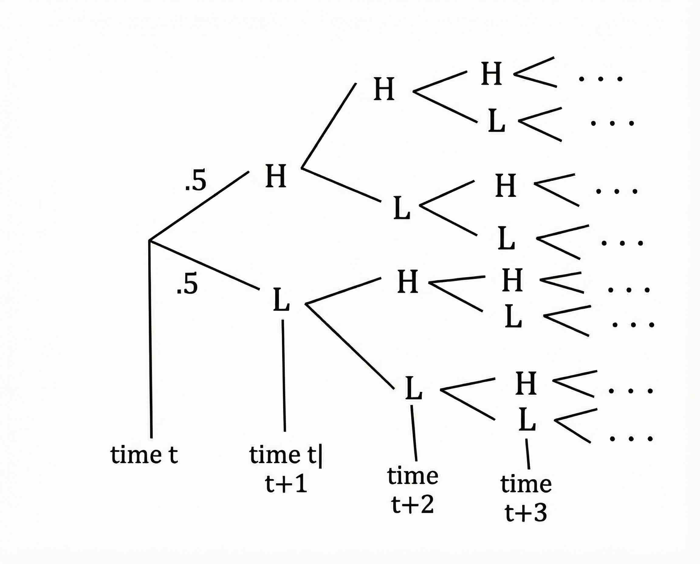
An example is an H/L process of dividends:
- Dividends are \(y_H\) with probability 0.5 and \(y_L\) with probability 0.5 (iid). Can denote these as \({\mathbb{P}_{}\left( {H} \right)} = {\mathbb{P}_{}\left( {L} \right)} = 0.5\)
- What is the expected present discounted value of payoffs? That is, \(p(Y_0) = \mathbb{E}_{t}\left[{\sum_{j=0}^{\infty} \beta^j Y_{t+j}} \; \middle| \; {Y_0} \right]\)?
The figure above shows how complicated this is to think through sequentially. But can we write down a recursive version of this under the assumption that the price should be only a function of the current state?
Define \(p_H\) and \(p_L\) as the prices in state \(H\) vs. \(L\). With this, we can write down a system of two equations and two unknowns.
\[ \begin{aligned} p_H &= y_H + \beta \mathbb{E}_{}\left[{p_i} \; \middle| \; {H} \right] = y_H + \beta \left[{\mathbb{P}_{}\left( {H} \right)} p_H + {\mathbb{P}_{}\left( {L} \right)} p_L\right]\\ p_L &= y_L + \beta \mathbb{E}_{}\left[{p_i} \; \middle| \; {L} \right] = y_L + \beta \left[{\mathbb{P}_{}\left( {H} \right)} p_H + {\mathbb{P}_{}\left( {L} \right)} p_L\right] \end{aligned} \]
Stack as vectors:
\[ \begin{aligned} p &\equiv \begin{bmatrix} p_H & p_L \end{bmatrix}\\ G &\equiv \begin{bmatrix} y_H & y_L \end{bmatrix}\\ A &\equiv \begin{bmatrix} {\mathbb{P}_{}\left( {H} \right)} & {\mathbb{P}_{}\left( {H} \right)} \\ {\mathbb{P}_{}\left( {L} \right)} & {\mathbb{P}_{}\left( {L} \right)} \end{bmatrix} \end{aligned} \]
Then rewrite the system of equations:
\[ p = G + \beta p A \]
Rearrange, being careful with the commutative rules of matrices:
\[ p(I - \beta A) = G \]
And assuming things are invertible:
\[ p = G (I - \beta A)^{-1} \]
In the more general case of a Markov chain, the \(A\) becomes the transpose of a Markov chain—as it does in the previous section. Here the columns are identical because the switches between \(L\) and \(H\) are iid.
To complete the solution, note that this \(p\) is a row vector, so if we set \(x_t\) as a column vector as above, \(x=\begin{bmatrix}1\\0 \end{bmatrix}\) if H, \(x=\begin{bmatrix}0\\1\end{bmatrix}\) if L, then we can calculate the price as \(p(x_t) = G(I - \beta A)^{-1} x_t\).
Stochastic Asset Pricing with Continuous State Spaces
Information Sets
- Conditional expectation \(\mathbb{E}(X | Y)\) means that in forming the expectation of \(X\), can use anything in \(Y\) as if known with certainty (i.e., not a random variable)
- \(\mathbb{E}_t(C_{t+1})\) is the abbreviation for \(\mathbb{E}(C_{t+1} \mid C_t, C_{t-1},C_{t-2}, \cdots \text{and anything else we know at t})\)
- If first-order Markov, then \(\mathbb{E}_t(C_{t+1}) = \mathbb{E}(C_{t+1} \mid C_t)\) (i.e., all info in last state)
- What to choose for the state? Think through necessary information set of an agent.
Properties of Expectations
Key: Expectation is a linear operator and can be over scalars, vectors, or matrices.
Some properties of expectations:
- Let \(a\) and \(b\) be scalar constants, and \(\{x_t\}\) and \(\{z_t\}\) be scalar random variables
- \({\mathbb{E}_{{t}}\left[ {a x_{t+1} + b z_{t+1}} \right]} = a {\mathbb{E}_{{t}}\left[ {x_{t+1}} \right]} + b {\mathbb{E}_{{t}}\left[ {z_{t+1}} \right]}\)
- But, be careful not to apply this for multiplication with other random variables:
- \({\mathbb{E}_{{t}}\left[ {x_{t+1} z_{t+1}} \right]} \neq {\mathbb{E}_{{t}}\left[ {x_{t+1}} \right]}{\mathbb{E}_{{t}}\left[ {z_{t+1}} \right]}\) in general (true if independent)
- \({\mathbb{E}_{{t}}\left[ {x_{t+1}^2} \right]} \neq \left({\mathbb{E}_{{t}}\left[ {x_{t+1}} \right]}\right)^{2}\) in general. Note \(x_{t+1}\) and \(x_{t+1}\) are never independent.
- As always, just be careful to keep the order (i.e., not commutative in general)
- Of course, if the information is known then the expectation is the value itself: \({\mathbb{E}_{{t}}\left[ {x_t} \right]} = {\mathbb{E}_{{}}\left[ {x_t | x_t} \right]} = x_t\)
- Law of iterated expectations: \({\mathbb{E}_{{t}}\left[ {{\mathbb{E}_{{t+1}}\left[ {x_{t+2}} \right]}} \right]} = {\mathbb{E}_{{t}}\left[ {x_{t+2}} \right]}\). Note: time \(t\) has less information than that of time \(t+1\).
Generalizing, let \(X_t\) and \(Z_t\) be vector random variables, and \(A\) and \(B\) be matrices or vectors:
- \({\mathbb{E}_{{t}}\left[ {A \cdot X_{t+1} + B \cdot Z_{t+1}} \right]} = A \cdot {\mathbb{E}_{{t}}\left[ {X_{t+1}} \right]} + B \cdot {\mathbb{E}_{{t}}\left[ {Z_{t+1}} \right]}\)
- These also all hold for any conditional expectation as well: \({\mathbb{E}_{{t}}\left[ {A \cdot X_{t+1} + B \cdot Z_{t+1} \,|\, Z_t, X_t} \right]} = A \cdot {\mathbb{E}_{{t}}\left[ {X_{t+1}\, |\, Z_t, X_t} \right]} + B \cdot {\mathbb{E}_{{t}}\left[ {Z_{t+1}\, |\, Z_t, X_t} \right]}\)
A Few Tricks with Normal Variables
- If a random variable \(z\) is distributed as a normal random variable with mean \(\mu\) and variance \(\sigma^2\), it is denoted
\[ z \sim N(\mu, \sigma^2) \]
- In terms of expectations, one can show that: \({\mathbb{E}_{{}}\left[ {z} \right]} = \mu\) and \({\mathbb{E}_{{}}\left[ {z^2} \right]} = \mu^2 + \sigma^2\)
- Let \(w \sim N(0,1)\) be a normalized random variable. Then you can show that
\[ z = \mu + \sigma w \]
- That is, you can convert any normal random variable to a linear function of a normalized one
- With multivariate normal random variable, \(q \in {\mathbb{R}}^n\), denote its distribution as \(q \sim N\left(\mu, \Sigma \right)\) where the mean \(\mu \in {\mathbb{R}}^n\) and \(\Sigma \in {\mathbb{R}}^{n\times n}\) is the variance-covariance matrix
- Keeping things simple, if the vector random variable has mean 0 and is independent (i.e., none of the components of the vector have any correlation) then we would write it as \(q \sim N(0_{n}, I_{n\times n})\)
Asset Pricing in Our State Space Model
The Deterministic Model
Recall: In the deterministic linear state space, we have
\[ \begin{aligned} &x_{t+1} = A \cdot x_t &&\text{(Evolution)}\\ &y_t = G \cdot x_t && \text{(Observation)} \end{aligned} \]
And the asset pricing formula under risk neutrality is:
\[ P_t = \sum_{j=0}^{\infty} \beta^j y_{t+j} = G(I-\beta\cdot A)^{-1}\cdot x_t \]
Making This a Stochastic Linear State Space
Add randomness \(w_{t+1}\), an \(m \times 1\) vector random variable:
\[ \begin{aligned} &x_{t+1} = A x_t+C \cdot w_{t+1} &&\text{(Evolution, stochastic)}\\ &y_t = G \cdot x_t &&\text{(Observation, still noise free)} \end{aligned} \]
where \(A\) is \(n \times n\) matrix, \(C\) is \(n \times m\) matrix, \(w_{t+1}\) are \(m \times 1\) matrices, \(x\) is \(n \times 1\) vector; \(G\) is \(1 \times n\) vector, \(y_t\) are scalars.
Note: \(w_{t+1}\) are independent, identically distributed variables; Gaussian of mean 0, covariance matrix \(I_{m \times m}\). Hence, \(\mathbb{E}(w_{it+1})=0\) for all \(i=1,\cdots m\), and
\[ \mathbb{E}(w_{it}w_{i't'})=\begin{cases} 1 & \text{if } i=i', t=t'\\ 0 & \text{otherwise}\end{cases} \]
Notice that:
\[ \mathbb{E}_t(x_{t+1})=\mathbb{E}_t(A\cdot x_t+Cw_{t+1})=A \cdot x_t+\underbrace{C\cdot \mathbb{E}_t(w_{t+1})}_{=0}=A\cdot x_t \]
\[ \mathbb{E}_t(x_{t+2}) = \mathbb{E}_t\left( A\underbrace{(Ax_t+Cw_{t+1})}_{x_{t+1}}+C\cdot w_{t+2}\right)=\mathbb{E}_t(A^2x_t+ACw_{t+1}+Cw_{t+2}) \]
\[ = A^2x_t+\underbrace{AC\mathbb{E}_t(w_{t+1})}_{=0}+\underbrace{C\mathbb{E}_t(w_{t+2})}_{=0}=A^2x_t \]
Repeat for \(t+3, \cdots\)
Forecasting Formulas:
\[ \mathbb{E}_t(x_{t+j}) = A^j x_t \quad \text{and} \quad \mathbb{E}_t\left(\sum_{j=0}^{\infty}\beta^jx_{t+j}\right) = (I-\beta\cdot A)^{-1}x_t \]
\[ \mathbb{E}_t(y_{t+j}) = G \cdot A^jx_t \quad \text{and} \quad \mathbb{E}_t\left(\sum_{j=0}^{\infty}\beta^jy_{t+j}\right) = G\cdot (I-\beta A)^{-1}x_t \]
Price of a Stochastic Dividend Stream
\[ p_t = \mathbb{E}_t\left(\sum_{j=0}^{\infty}\beta^j y_{t+j}\right) + \text{possible bubble} = G(I-\beta A)^{-1}x_t + \text{possible bubble} \]
Or, recursively:
\[ p_t = \underbrace{y_t}_{\substack{\text{dividend}\\\text{today}}} + \beta \cdot \underbrace{\mathbb{E}_t(p_{t+1})}_{\substack{\text{expectation}\\\text{of price}\\\text{tomorrow}}} \]
Method (Guess and Verify):
Guess \(p_t = H \cdot x_t\), where \(H\) is \(1 \times n\) vector to be determined, \(x\) is \(n \times 1\) vector.
Substitute into equation:
\[ H \cdot x_t = y_t+\beta \cdot \mathbb{E}_t\left(Hx_{t+1}\right) \]
\[ H \cdot x_t = G \cdot x_t + \beta H \mathbb{E}_t(A\cdot x_t + C \cdot w_{t+1}) = G\cdot x_t + \beta H A x_t \]
To hold for any \(x_t\):
\[ H(I-\beta A) = G \implies H = G(I-\beta A)^{-1} \]
Therefore:
\[ \boxed{p_t = G(I-\beta A)^{-1} x_t} \]
Note:
- This is consistent with the EPDV calculation
- Same formula as without random \(w_{t+1}\)
Forecast Errors
How far off are the agent’s forecasts of \(t+1\) given time \(t\) information? To do a simple example:
- Let \(x_{t+1} = x_t + \sigma w_{t+1}\)
- With \(w_{t+1} \sim N(0,1)\). That is, \({\mathbb{E}_{{t}}\left[ {w_{t+1}} \right]} = 0\) and \({\mathbb{E}_{{t}}\left[ {w_{t+1}^2} \right]} = 1\).
- This is a trivial linear-Gaussian-state space.
The expected forecast error is:
\[ {\mathbb{E}_{{t}}\left[ {FE_{t+1}} \right]} \equiv {\mathbb{E}_{{t}}\left[ {x_{t+1} - {\mathbb{E}_{{t}}\left[ {x_{t+1}} \right]}} \right]}= {\mathbb{E}_{{t}}\left[ {x_{t+1}} \right]} - {\mathbb{E}_{{t}}\left[ {x_{t+1}} \right]} = 0 \]
No systematic error. What about the variance of the forecast errors?
The variance of a random variable \(z_t\) is defined as \(\mathbb{V}_t\left(z_{t+1}\right) \equiv {\mathbb{E}_{{t}}\left[ {z_{t+1}^2} \right]} - \left({\mathbb{E}_{{t}}\left[ {z_{t+1}} \right]}\right)^2\).
So to find the variance of the forecast error:
\[ \begin{aligned} \mathbb{V}_t(FE_{t+1}) &= {\mathbb{E}_{{t}}\left[ {FE_{t+1}^2} \right]} - \left({\mathbb{E}_{{t}}\left[ {FE_{t+1}} \right]}\right)^2\\ &= {\mathbb{E}_{{t}}\left[ {\left(x_{t+1} - {\mathbb{E}_{{t}}\left[ {x_{t+1}} \right]}\right)^2} \right]} - 0\\ &= {\mathbb{E}_{{t}}\left[ {\left(x_t + \sigma w_{t+1} - {\mathbb{E}_{{t}}\left[ {x_t + \sigma w_{t+1}} \right]}\right)^2} \right]}\\ &= {\mathbb{E}_{{t}}\left[ {\left(\sigma w_{t+1}\right)^2} \right]} = \sigma^2 \end{aligned} \]
Linear Gaussian State Space Example
- On average, a worker’s productivity, \(z_t\), adds a random draw of \(N(\alpha, \sigma^2)\) each period
- Firm productivity \(q_t\) adds \(\gamma\) each period, which is deterministic
- Wages are a linear combination: \(W_t = \theta z_t+(1-\theta)q_t\)
Setup in Linear Gaussian form:
Guess state: \(x_t = \begin{bmatrix} z_t \\ q_t \\ 1 \end{bmatrix}\)
Note: if \(w_{t+1} \sim N(0,1)\), then
\[ \alpha + \sigma w_{t+1} \sim N(\alpha, \sigma^2) \]
The state space model is then:
\[ \underbrace{\begin{bmatrix}z_{t+1}\\ q_{t+1} \\1\end{bmatrix}}_{x_{t+1}} = \underbrace{\begin{bmatrix}1&0&\alpha \\ 0&1&\gamma\\0&0&1 \end{bmatrix}}_{A} \underbrace{\begin{bmatrix}z_t\\ q_t\\ 1 \end{bmatrix}}_{x_t}+ \underbrace{\begin{bmatrix}\sigma \\ 0 \\0 \end{bmatrix}w_{t+1}}_{C \cdot w_{t+1}} \]
\[ W_t = \begin{bmatrix}\theta& 1-\theta & 0\end{bmatrix} \begin{bmatrix}z_t \\ q_t \\1 \end{bmatrix} = G \cdot x_t \]
What is the expected PDV of human capital? (i.e., stochastic version of the permanent income calculations)
\[ {\mathbb{E}_{{t}}\left[ {\sum_{j=0}^{\infty} \beta^j y_{t+j}} \right]} = G(I - \beta A)^{-1}x_t \]
Appendices
Stochastic Bubbles
To isolate the bubble term, consider the special case where \(y_t = 0\) for all \(t\).
We want to solve \(p_t = \beta \mathbb{E}_t(p_{t+1})\), where \(\beta = \frac{1}{1+r}\).
Guess: \(p_t = C_t \beta^{-t}\), where \(C_t\) is a random variable, and \(\{C_t\}\) is a martingale, that is, satisfies \(\mathbb{E}_t{(C_{t+1})} = C_t\) (i.e., best forecast of future value is today’s value, e.g., random walk).
To verify \(p_t = \beta \mathbb{E}_t(p_{t+1})\), substitute our guess:
\[ C_t \beta^{-t} = \beta \cdot \mathbb{E}_t(\beta^{-(t+1)}C_{t+1}) = \beta^{-t}\cdot \mathbb{E}_t(C_{t+1}) = \beta^{-t}C_t \]
Verified that \(p_t = C_t \beta ^{-t}\) satisfies the equation.
Example:
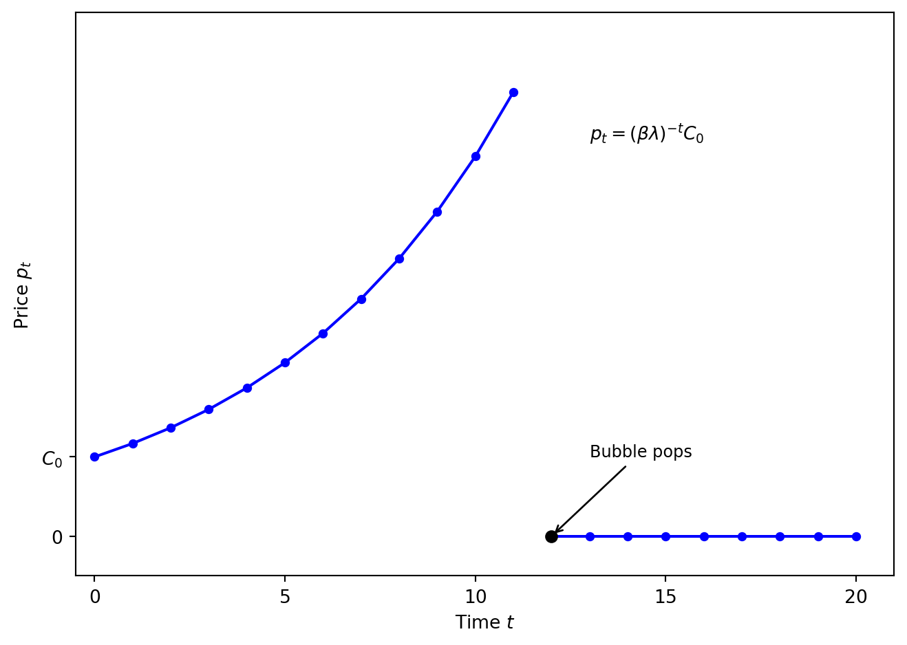
\[ C_{t+1} = \begin{cases}\lambda^{-1}C_t & \text{with probability } \lambda \in (0,1)\\0 & \text{with probability } 1-\lambda\end{cases} \]
- Note: \(\mathbb{E}_t(C_{t+1}) = \lambda\cdot(\lambda^{-1}C_t)+0 = C_t\), so this is a martingale
- Note that if at some point \(C_{t+j} = 0\), then \(C_{t+j+1} = 0\), etc. (i.e., the bubble has popped)
- From any \(C_0\):
\[ C_{t} = \begin{cases} \lambda^{-t}C_0 & \text{if bubble has not popped}\\ 0 & \text{if the bubble has popped}\end{cases} \]
\[ p_t = \begin{cases} \beta^{-t}\cdot \lambda^{-t} \cdot C_0 = (\beta\lambda)^{-t}C_0 & \text{until popped}\\ 0 & \text{after the bubble has popped}\end{cases} \]