Permanent Income Model
Honours Intermediate Macro
Consumption smoothing, Euler equations, and the permanent income hypothesis
Permanent Income Model
Basic Setup
The permanent income hypothesis started with Friedman (1957) in the 1950s, and was extended to rational expectations by Hall (1978) in the late 1970s.
- Agent has an (exogenous) deterministic income \(\left\{{y_{t+j}}\right\}_{j=0}^{\infty}\) and (initially exogenous) savings \(F_t\).
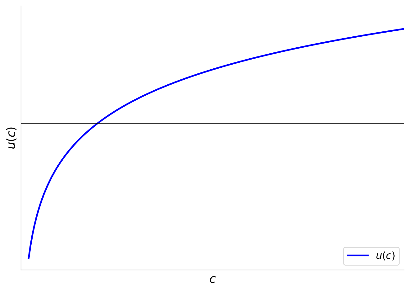
- Chooses sequence of consumption to maximize the PDV of utility of consumption \(u(c_t)\) for all \(t\).
- That is: at time \(t\), solves (given exogenous \(\left\{{y_{t+j}}\right\}\) and \(F_t\)):
\[ \max_{\left(c_{t+j}\right)_{j=0}^{\infty}} \left\{\sum_{j=0}^{\infty} \beta^j u(c_{t+j})\right\} \]
subject to the lifetime budget constraint:
\[ \sum_{j=0}^{\infty} \underbrace{\left(\frac{1}{R}\right)^j}_{\substack{\text{discounting with} \\ \text{interest rate}}} \left(\underbrace{y_{t+j}}_{\text{labor income}} - \underbrace{c_{t+j}}_{\text{consumption}}\right) + \underbrace{F_t}_{\text{assets}} = 0 \tag{1}\]
where \(\beta \in (0,1)\) is the discount factor and \(R > 1\) is the gross interest rate. Assets are used to finance any difference between consumption and labor income over the lifetime.
Lagrangian
\[ \mathcal{L} = \sum_{j=0}^{\infty} \beta^j u(c_{t+j}) + \lambda \left[\sum_{j=0}^{\infty}\left(\frac{1}{R}\right)^j \left(y_{t+j}-c_{t+j}\right) + F_t\right] \]
Note:
- Infinite number of variables \(\left\{{c_{t+j}}\right\}_{j=0}^{\infty}\) and one constraint
- The constraint is a lifetime budget constraint
First Order Necessary Condition (FONC):
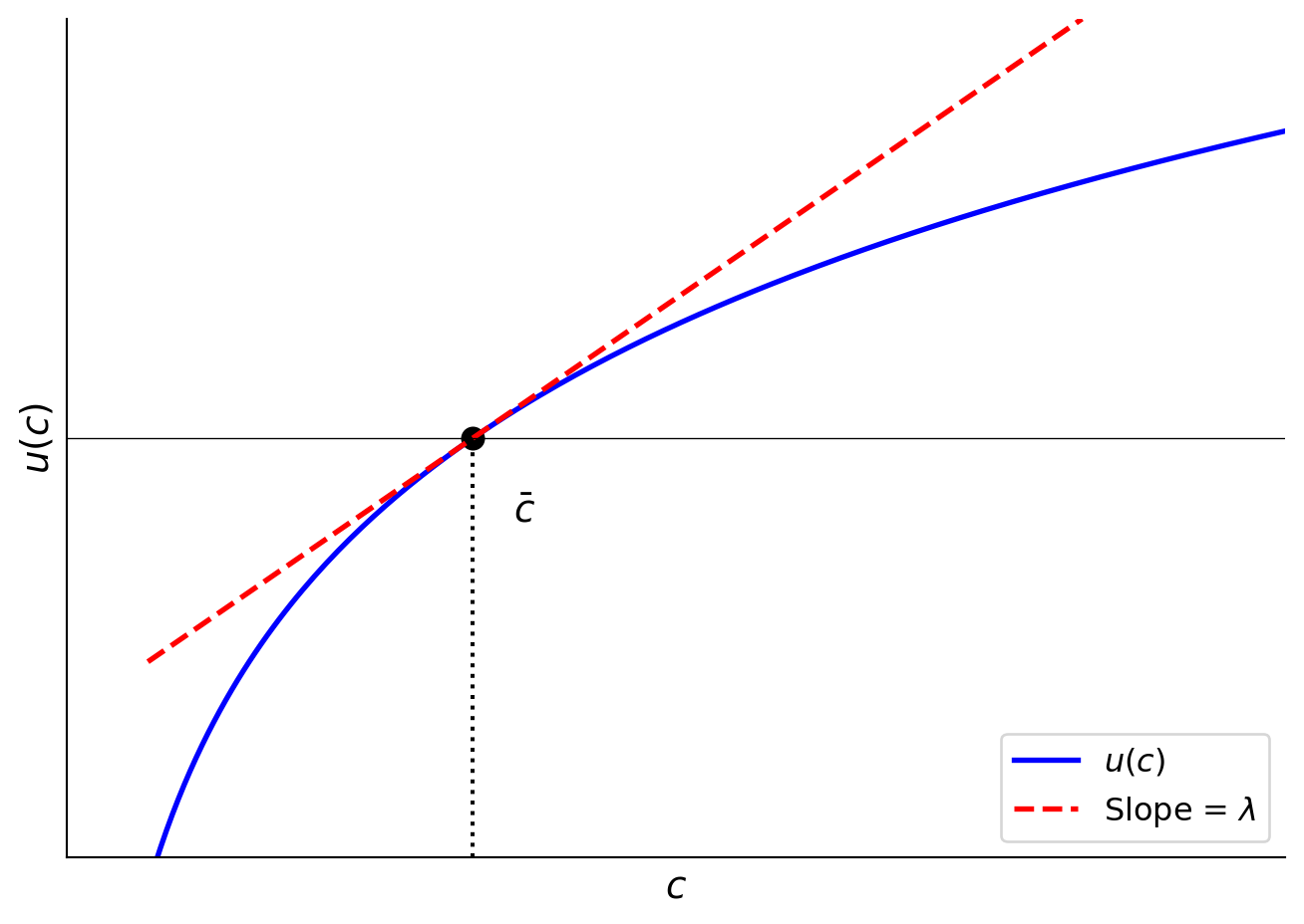
\[ c_{t+j}: \beta^j u'(c_{t+j}) - \lambda R^{-j} = 0 \quad \Rightarrow \quad u'(c_{t+j}) = \left(\frac{1}{\beta R}\right)^j \cdot \lambda, \quad \forall j \]
Example: If \(R = 1/\beta\), then \(u'(c_{t+j}) = \left(\frac{1}{\beta R}\right)^j \cdot \lambda = \lambda\) for all \(j\). The slope at \(c_{t+j}\) equals \(\lambda\), which means the marginal utility is constant. Therefore \(c_{t+j}\) is constant for all \(j\), giving us \(\bar{c} = c_{t+j} = u'^{-1}(\lambda)\).
Budget constraint: From Equation 1,
\[ \sum_{j=0}^{\infty} R^{-j} c_{t+j} = F_t + \sum_{j=0}^{\infty} R^{-j} y_{t+j} \]
Example: If \(R = 1/\beta\), solve for \(\bar{c}\):
\[ \bar{c} = \underbrace{(1-\beta)}_{\substack{\text{marginal propensity} \\ \text{to consume} \\ \text{out of wealth}}} \left[\underbrace{\sum_{j=0}^{\infty} \beta^j y_{t+j}}_{\substack{\text{PDV of} \\ \text{human wealth}}} + \underbrace{F_t}_{\substack{\text{Financial} \\ \text{wealth}}}\right] \]
Manipulating the Budget Constraint
At time \(t\):
\[ \sum_{j=0}^{\infty} R^{-j} y_{t+j} + F_t = \sum_{j=0}^{\infty} R^{-j} c_{t+j} \]
At time \(t+1\):
\[ \sum_{j=0}^{\infty} R^{-j} y_{t+j+1} + F_{t+1} = \sum_{j=0}^{\infty} R^{-j} c_{t+j+1} \]
Multiply the time \(t+1\) equation by \(1/R\) and write out terms.
At time \(t\):
\[ F_t + y_t + R^{-1}y_{t+1} + R^{-2}y_{t+2} + \cdots = c_t + R^{-1}c_{t+1} + R^{-2}c_{t+2} + \cdots \]
At time \(t+1\) (multiplied by \(1/R\)):
\[ R^{-1}F_{t+1} + R^{-1}y_{t+1} + R^{-2}y_{t+2} + \cdots = R^{-1}c_{t+1} + R^{-2}c_{t+2} + \cdots \]
Subtracting equations, most terms cancel out:
\[ F_t - R^{-1}F_{t+1} + y_t = c_t \]
Therefore:
\[ \underbrace{F_{t+1}}_{\substack{\text{next period's} \\ \text{wealth}}} = \underbrace{R}_{\substack{\text{gross interest} \\ \text{rate}}} \left[\underbrace{F_t}_{\substack{\text{this period's} \\ \text{wealth}}} + \underbrace{y_t - c_t}_{\text{savings}}\right] \tag{2}\]
Note: Sometimes we define \(1 + \underbrace{r}_{\substack{\text{net interest} \\ \text{rate}}} \equiv \underbrace{R}_{\substack{\text{gross interest} \\ \text{rate}}}\).
So an equivalent form of the Permanent Income Hypothesis is:
\[ \max_{\left\{{c_t, F_{t+1}}\right\}_{t=0}^{\infty}} \left\{\sum_{t=0}^{\infty} \beta^t u(c_t)\right\}, \quad F_0 \text{ given} \]
\[ \,\text{s.t.}\,F_{t+1} = R(F_t + y_t - c_t), \quad t = 0, \ldots, \infty \]
Note:
- In addition, it will require a variation of \(\lim_{T \to \infty} \beta^{T+1} F_{T+1} \geq 0\) (Transversality Condition, No Ponzi-condition, etc.). Agent cannot asymptotically have debt. We will ignore this constraint for now.
- There are period-by-period budget constraints.
- Chooses consumption and savings for next period.
- \(R\) is the gross rate of return on assets.
Lagrangian with Period-by-Period Constraints
Lagrangian for Lagrange multipliers \(\hat{\lambda}_t\) on budgets:
\[ \mathcal{L} = \sum_{t=0}^{\infty} \beta^t u(c_t) + \sum_{t=0}^{\infty} \hat{\lambda}_t \left[R(F_t + y_t - c_t) - F_{t+1}\right] \]
where \(\hat{\lambda}_t\) is the Lagrange multiplier on the budget constraint at time \(t\).
Writing out portions of the sequence:
\[ \mathcal{L} = \cdots + \beta^t u(c_t) + \beta^{t+1} u(c_{t+1}) + \hat{\lambda}_t[R(F_t + y_t - c_t) - F_{t+1}] + \hat{\lambda}_{t+1}[R(F_{t+1} + y_{t+1} - c_{t+1}) - F_{t+2}] + \cdots \]
FOC(\(c_t\)):
\[ 0 = \beta^t u'(c_t) - \hat{\lambda}_t R \quad \Rightarrow \quad \hat{\lambda}_t R = \beta^t u'(c_t) \tag{3}\]
FOC(\(F_{t+1}\)):
\[ 0 = -\hat{\lambda}_t + \hat{\lambda}_{t+1} R \quad \Rightarrow \quad \frac{\hat{\lambda}_{t+1}}{\hat{\lambda}_t} = \frac{1}{R} \tag{4}\]
Take Equation 3 at time \(t+1\) and at time \(t\):
\[ \frac{\beta^{t+1}}{\beta^t} \frac{u'(c_{t+1})}{u'(c_t)} = \frac{\hat{\lambda}_{t+1} \cdot R}{\hat{\lambda}_t \cdot R} \]
Use Equation 4:
\[ \beta \frac{u'(c_{t+1})}{u'(c_t)} = \frac{1}{R} \]
Therefore:
\[ u'(c_t) = \beta R \, u'(c_{t+1}) \quad \text{(Euler equation)} \tag{5}\]
Note in Equation 3, let \(\lambda_t \beta^t \equiv \hat{\lambda}_t\) (just a new definition for \(\lambda_t\)), then \(\lambda_t \beta^t R = \beta^t u'(c_t)\), so \(u'(c_t) = R \lambda_t\). These are present-value Lagrange multipliers and can be stationary instead of exponentially shrinking (i.e., if \(c_t \to \bar{c}\)).
Interpreting the Euler Equation
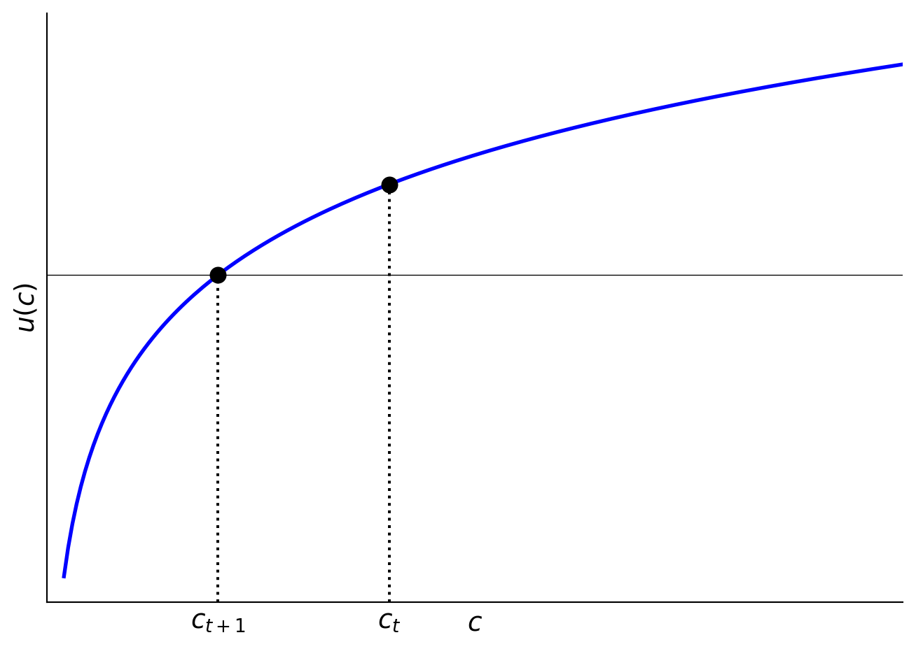
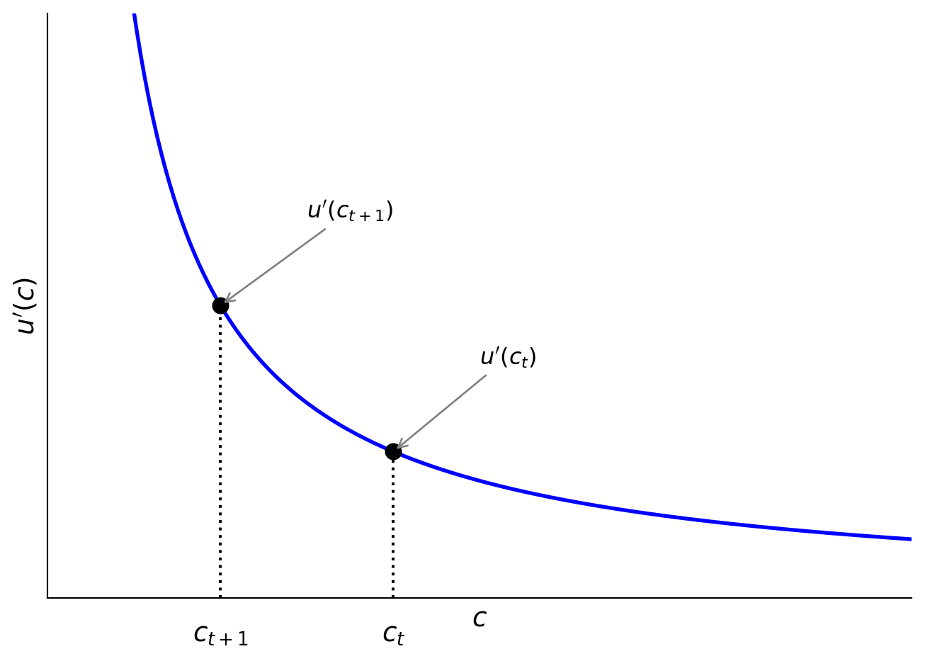
Figure 3 shows what it might be like to have the utility of consumption of two different \(c_t\) and \(c_{t+1}\). The corresponding Figure 4 shows the intertemporal tradeoff of lowering \(c_t\) to increase \(c_{t+1}\), which has higher marginal utility of consumption.
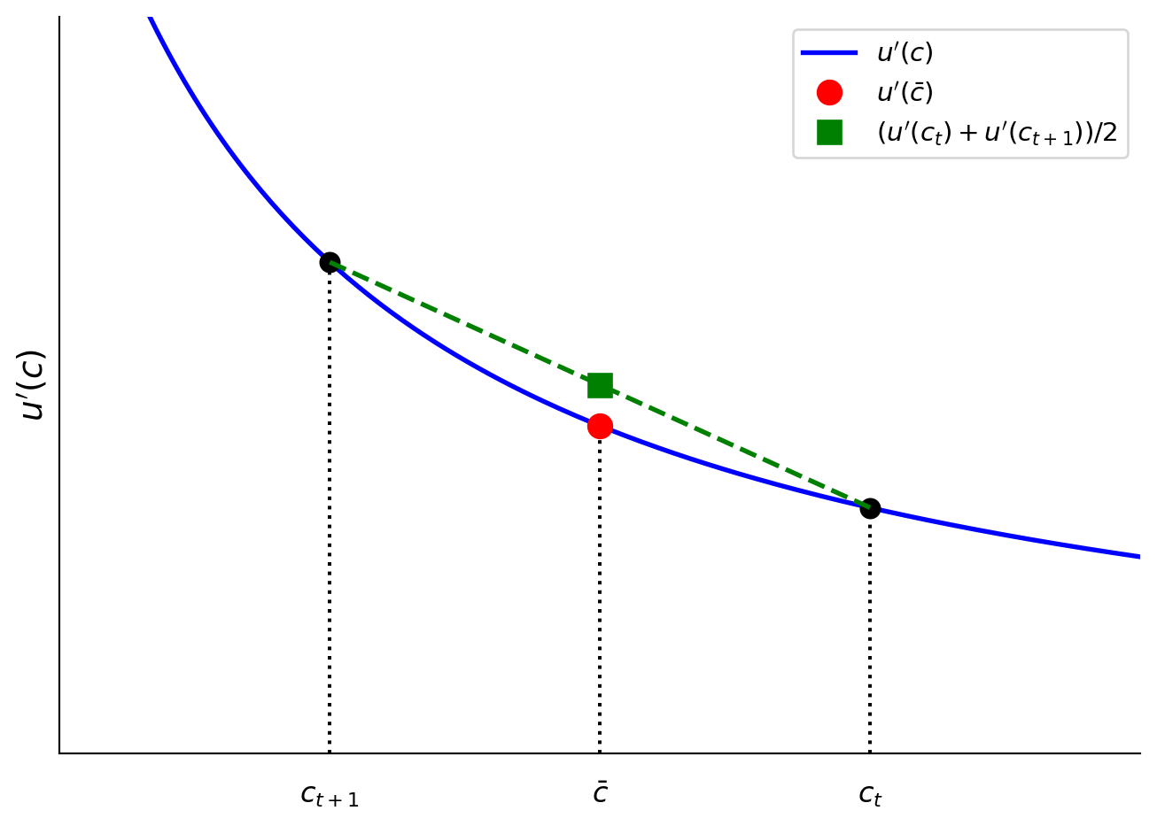
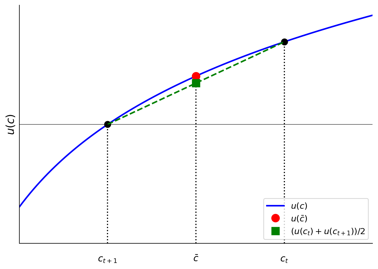
Figure 5 shows the simple case of \(\beta R = 1\) and two periods. If you take the average of the two periods’ consumption for both, it has a lower marginal utility of consumption—which corresponds to a higher utility as we see in Figure 6.
Rescaling Lagrange Multipliers
In general, Lagrange multipliers can be rescaled and redefined to make either math or interpretation easier. One way to think of this is to notice that both problems
\[ \arg\max_x f(x) \quad \,\text{s.t.}\,g(x) = 0 \qquad \text{and} \qquad \arg\max_x f(x) \quad \,\text{s.t.}\,A \cdot g(x) = 0 \]
have the same solution \(x^*\) for all \(A \neq 0\) (which, crucially, cannot depend on \(x\)).
What this means is that the FONCs using the two Lagrange multipliers would lead to the same \(x\) solutions. That is, solving the FONC of
\[ \mathcal{L}_1 \equiv f(x) + \lambda_1 g(x) \]
and
\[ \mathcal{L}_2 \equiv f(x) + \lambda_2 A g(x) \]
would lead to different \(\lambda_1 \neq \lambda_2\) solutions, but would have the same \(x\).
Because of this, we may sometimes skip rescaling steps like the above and write down the Lagrange multipliers directly as \(\lambda_2\) from \(\max_x f(x) \,\text{s.t.}\,g(x) = 0\) directly, skipping the multiplication by \(A\) as above.
Alternative Lagrangian (Generally Preferred)
Directly group the \(\lambda_t\) inside the sum:
\[ \mathcal{L} = \sum_{t=0}^{\infty} \beta^t \left[u(c_t) + \lambda_t \left[R(F_t + y_t - c_t) - F_{t+1}\right]\right] \]
Inside the sum, \(\lambda_t\) is the same as \(\lambda_t \beta^t \equiv \hat{\lambda}_t\).
\[ \mathcal{L} = \cdots + \beta^t[u(c_t) + \lambda_t[R(F_t + y_t - c_t) - F_{t+1}]] + \beta^{t+1}[u(c_{t+1}) + \lambda_{t+1}[R(F_{t+1} + y_{t+1} - c_{t+1}) - F_{t+2}]] + \cdots \]
\(\partial/\partial c_t\):
\[ \beta^t[u'(c_t) - \lambda_t R] = 0 \quad \Rightarrow \quad u'(c_t) = R \lambda_t \tag{6}\]
\(\partial/\partial F_{t+1}\):
\[ -\beta^t \lambda_t + \beta^{t+1} R \lambda_{t+1} = 0 \quad \Rightarrow \quad \frac{\lambda_{t+1}}{\lambda_t} = \frac{1}{\beta R} \tag{7}\]
Take Equation 6 divided at \(t\) and \(t+1\):
\[ \frac{u'(c_{t+1})}{u'(c_t)} = \frac{\lambda_{t+1}}{\lambda_t} \quad \text{(These are called "present-value Lagrange multipliers")} \]
Using Equation 7:
\[ \frac{u'(c_{t+1})}{u'(c_t)} = \frac{1}{\beta R} \]
Therefore:
\[ u'(c_t) = \beta R \, u'(c_{t+1}) \quad \text{(Identical Euler equation)} \]
Recall that budget constraints need to be held. Could use either the \(\infty\) number of period-by-period constraints, or lifetime budget constraint:
\[ \sum_{j=0}^{\infty} \left(\frac{1}{R}\right)^j c_{t+j} = F_t + \sum_{j=0}^{\infty} \left(\frac{1}{R}\right)^j y_{t+j} \]
With this and the Euler equation, we may not need to solve for intermediate \(F_{t+1}\) choices, though we could at the end.
Finite Horizon
Finite Horizon (Formally)
Die at \(T > 0\), i.e., no utility from consumption after \(T\). Need additional constraint so they do not die in debt:
\[ \max_{\left\{{c_t, F_{t+1}}\right\}_{t=0}^T} \left\{\sum_{t=0}^T \beta^t u(c_t)\right\} \]
\[ \,\text{s.t.}\,F_{t+1} = R(F_t + y_t - c_t) \quad \text{for } t = 0, \ldots, T \]
\[ F_{T+1} \geq 0 \quad \text{(weakly positive assets at death)} \]
\[ F_0 \text{ given} \]
Multipliers: Use present value constraints:
- \(\lambda_0, \ldots, \lambda_T\) on first constraints
- \(\lambda_{T+1}\) on last constraint
i.e., total of \(T+2\) constraints.
\[ \mathcal{L} = \sum_{t=0}^T \beta^t \left[u(c_t) + \lambda_t[R(F_t + y_t - c_t) - F_{t+1}]\right] + \underbrace{\beta^{T+1} \lambda_{T+1}}_{\substack{\text{terminal constraint} \\ \text{present value} \\ \hat{\lambda}_{T+1} \equiv \beta^{T+1}\lambda_{T+1}}} F_{T+1} \]
FOC(\(c_t\)):
\[ u'(c_t) = R \lambda_t, \quad \text{for } t = 0, \ldots, T \]
i.e., die at \(T+1\), no utility. Therefore:
\[ \frac{u'(c_{t+1})}{u'(c_t)} = \frac{\lambda_{t+1}}{\lambda_t}, \quad \forall t \leq T-1 \]
FOC(\(F_{t+1}\)) for \(t < T\):
\[ 0 = -\lambda_t + \lambda_{t+1} \beta R \quad \Rightarrow \quad \lambda_t = \beta R \lambda_{t+1} \tag{8}\]
FOC(\(F_{T+1}\)):
\[ 0 = -\beta^T \lambda_T + \beta^{T+1} \lambda_{T+1} \quad \Rightarrow \quad \lambda_T = \beta \lambda_{T+1} \tag{9}\]
With \(\beta^{T+1} F_{T+1} \lambda_{T+1} = 0\), \(\lambda_{T+1} \geq 0\) (since inequality constraint, need complementary slackness).
Does the Terminal Constraint Bind?
By Contradiction: Assume not, i.e., \(\lambda_{T+1} = 0\) (which implies \(F_{T+1} > 0\)). Then from Equation 9, \(\lambda_T = 0\), and from Equation 8, \(\lambda_t = 0\) for all \(t\).
So if it does not bind at time \(T+1\), it never binds. Only possible if \(u'(c_t) = 0\) for all \(t\), which is a contradiction. Hence, \(F_{T+1} = 0\) (unless there is a budget-feasible satiation point where \(u'(c_t) = 0\) for all \(t\), e.g., quadratic utility with enormous budgets).
Period Budget Constraints and Lifetime Budget Constraints
See the derivation in which takes the
\[ F_{t+1} = R(F_t + y_t - c_t), \quad \forall t = 0, \ldots, T \]
\[ F_{T+1} = 0 \]
and finds
\[ \underbrace{\sum_{j=0}^{T-t} R^{-j} c_{t+j}}_{\substack{\text{PDV of} \\ \text{consumption}}} = \underbrace{\sum_{j=0}^{T-t} R^{-j} y_{t+j}}_{\substack{\text{PDV of} \\ \text{labor income}}} + \underbrace{F_t}_{\substack{\text{Financial} \\ \text{wealth}}} \]
If \(T \to \infty\), then we see that this is identical to Equation 1. This result provides somewhat of the opposite direction to Section 1.3, where we show that the sequential constraints imply the lifetime budget constraint (under conditions on what happens to \(F_T\) as \(T \to \infty\)).
Summary of Equations
\[ u'(c_t) = \beta R \, u'(c_{t+1}), \quad \forall t = 0, \ldots, T-1 \tag{10}\]
\[ F_{t+1} = R(F_t + y_t - c_t), \quad \forall t = 0, \ldots, T \tag{11}\]
\[ F_{T+1} = 0, \quad F_0 \text{ given} \tag{12}\]
Given: \(F_0\), \(\left\{{y_t}\right\}_{t=0}^T\), find \(\left\{{c_t}\right\}_{t=0}^T\). How?
In general, we need computers to solve this problem. See for an example algorithm.
Examples
Assume we have utility as follows:
\[ u(c) = \log(c), \quad T \leq \infty \quad \Rightarrow \quad u'(c) = \frac{1}{c} \]
From the Euler equation:
\[ \frac{1}{c_t} = \beta R \frac{1}{c_{t+1}} \quad \Rightarrow \quad c_{t+1} = \beta R c_t, \quad \text{for } t = 0, \ldots, T \]
\[ \Rightarrow c_t = (\beta R)^t c_0 \]
Find \(c_0\) from the lifetime budget.
Example 1: Infinite Horizon with Growing Income
\(T = \infty\), \(y_t = \delta^t y_0\), \(F_0 = 0\)
Use budget:
\[ 0 = \sum_{j=0}^{\infty} R^{-j} \left((\beta R)^j c_0 - \delta^j y_0\right) \]
\[ \Rightarrow c_0 \sum_{j=0}^{\infty} \beta^j = \sum_{j=0}^{\infty} \left(\frac{\delta}{R}\right)^j y_0 \quad \text{(assume } \left|\frac{\delta}{R}\right| < 1\text{)} \]
Therefore:
\[ c_0 = (1-\beta) \cdot \left(\frac{1}{1-\frac{\delta}{R}}\right) y_0 \]
Example 2: Finite Horizon with Growing Income
\(T < \infty\), \(y_t = \delta^t y_0\), \(F_0 = 0\)
\[ 0 = \sum_{j=0}^T R^{-j} \left((\beta R)^j c_0 - \delta^j y_0\right) \]
\[ \Rightarrow c_0 \sum_{j=0}^T \beta^j = \sum_{j=0}^T \left(\frac{\delta}{R}\right)^j y_0 \]
Use partial geometric sums:
\[ \frac{1-\beta^{T+1}}{1-\beta} c_0 = \left[\frac{1-\left(\frac{\delta}{R}\right)^{T+1}}{1-\frac{\delta}{R}}\right] y_0 \]
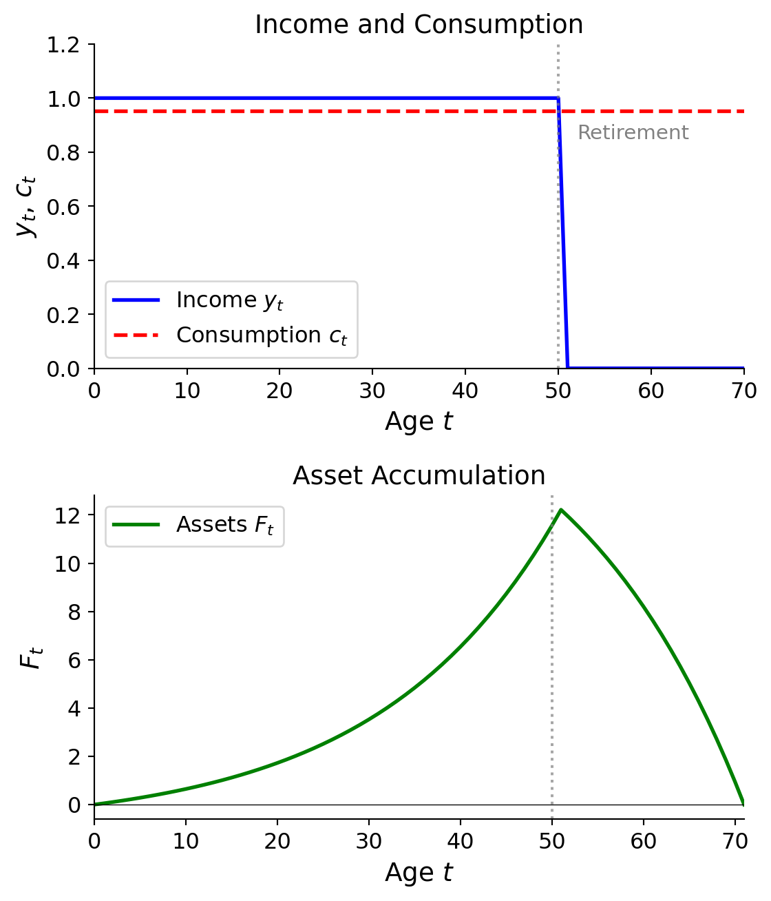
Example 3: Retirement
\(F_0 = 0\), \(T = 70\), \(y_t = \begin{cases} \delta^t y_0, & t = 0, \ldots, 50 \\ 0, & t = 51, \ldots, 70 \end{cases}\)
i.e., stop working at 50, die at 70, where \(t\) is the age.
Put into budget:
\[ c_0 \sum_{t=0}^{70} R^{-t} (\beta R)^t = \sum_{t=0}^{50} \left(\frac{\delta}{R}\right)^t \cdot y_0 \]
\[ \Rightarrow c_0 \cdot \frac{1-\beta^{71}}{1-\beta} = \frac{1-\left(\frac{\delta}{R}\right)^{51}}{1-\frac{\delta}{R}} y_0 \]
Solution:
\[ c_0 = \frac{1-\beta}{1-\beta^{71}} \cdot \frac{1-\left(\frac{\delta}{R}\right)^{51}}{1-\frac{\delta}{R}} \cdot y_0 \]
\[ c_t = (\beta R)^t \cdot c_0 \]
\[ F_{t+1} = R(F_t + y_0 \delta^t - (\beta R)^t \cdot c_0) \]
Can substitute for \(c_0\) to get lifetime savings.
Example: Special Case \(\beta R = 1\)
\(\beta R = 1 \Rightarrow c_t = c_0\) for all \(t\). Constant consumption.
Example: Growing Income and Early Borrowing
Now consider the case where income grows over time (\(\delta > 1\)). With \(\beta R = 1\), consumption is still constant, but since income starts low and grows, the agent must borrow early in life to smooth consumption. Assets become negative initially, then turn positive as the agent pays off debt and saves for retirement.
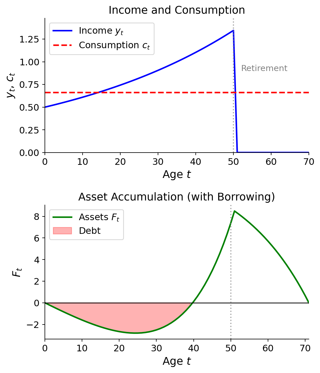
Key observations:
- Early life (borrowing phase): Income is below consumption, so \(y_t - c_t < 0\). The agent borrows (\(F_t < 0\)).
- Mid-career (debt repayment and saving): Income rises above consumption. The agent pays off debt, then accumulates savings.
- Retirement (dissaving): Income drops to zero. The agent draws down savings to maintain consumption.
This illustrates why access to credit markets is valuable: without borrowing, young agents with growing income profiles would be forced to consume less than optimal early in life.
Appendices
Shooting Method
An iterative approach:
- If we knew \(c_0\), then since we know \(F_0\):
- Use Equation 10 to find \(c_1\)
- Use Equation 11 to find \(F_1\)
- Repeat for \(\left\{{c_2, F_2}\right\}\), etc. to \(T-1\)
- Use Equation 11 with \(c_T\), \(F_T\) to get \(F_{T+1}\)
- Check Equation 12 satisfied or not.
Convergence of the iterative solution:
- Guess \(c_0\)
- Find sequence using the above steps to get \(F_{T+1}\)
- If \(F_{T+1} > 0\), raise \(c_0\) and try again. If \(F_{T+1} < 0\), lower \(c_0\) and try again.
- Stop when \(F_{T+1} \approx 0\)
Lifetime Budget Constraint Derivation
We could use:
\[ F_{t+1} = R(F_t + y_t - c_t), \quad \forall t = 0, \ldots, T \]
\[ F_{T+1} = 0 \]
Alternatively, work backwards from \(T\):
\[ 0 = R(F_T + y_T - c_T) \quad \Rightarrow \quad c_T - y_T = F_T \]
Then for \(T-1\):
\[ F_T = R(F_{T-1} + y_{T-1} - c_{T-1}) \]
Using the previous result: \(c_T - y_T = R(F_{T-1} + y_{T-1} - c_{T-1})\)
\[ \Rightarrow F_{T-1} = c_{T-1} - y_{T-1} + \frac{1}{R}(c_T - y_T) \]
At \(t = T-2\):
\[ F_{T-1} = R(F_{T-2} + y_{T-2} - c_{T-2}) \]
\[ \Rightarrow c_{T-1} - y_{T-1} + \frac{1}{R}(c_T - y_T) = R(F_{T-2} + y_{T-2} - c_{T-2}), \text{ etc.} \]
Finally, repeat until \(F_0\):
\[ F_0 = \sum_{t=0}^T \left(\frac{1}{R}\right)^t (c_t - y_t) \]
More generally, starting at any \(t\):
\[ \underbrace{\sum_{j=0}^{T-t} R^{-j} c_{t+j}}_{\substack{\text{PDV of} \\ \text{consumption}}} = \underbrace{\sum_{j=0}^{T-t} R^{-j} y_{t+j}}_{\substack{\text{PDV of} \\ \text{labor income}}} + \underbrace{F_t}_{\substack{\text{Financial} \\ \text{wealth}}} \]
Compare to the lifetime budget constraint Equation 1.
References
Friedman, Milton. 1957. A Theory of the Consumption Function. Princeton University Press.
Hall, Robert E. 1978. “Stochastic Implications of the Life Cycle-Permanent Income Hypothesis: Theory and Evidence.” Journal of Political Economy 86 (6): 971–87.