Math Review
Honours Intermediate Macro
Review of linear algebra, functional equations, optimization, and probability
Linear Algebra
Vectors
- Notation: \(x \in {\mathbb{R}}^{n}\) is a vector of \(n\) reals
- Vector \(x = \begin{bmatrix} x_1 \\ x_2 \\ \vdots \\ x_n\end{bmatrix}\) (column vector)
- Element: \(x_i\) is the \(i\)th element of the vector \(x\)
- Transpose: \(x^\top = \begin{bmatrix} x_1 & x_2 & \ldots & x_n\end{bmatrix}\) (row vector)
Vector Operations
Addition: \((x + y)_i = x_i + y_i\)
\[ \begin{bmatrix} 1 \\ 2 \\ 3 \end{bmatrix} + \begin{bmatrix} 4 \\ 5 \\ 6 \end{bmatrix} = \begin{bmatrix} 5 \\ 7 \\ 9 \end{bmatrix} \]
Scalar Multiplication: \((\alpha x)_i = \alpha x_i\) for \(\alpha \in {\mathbb{R}}\)
- Commutative: \(\alpha x = x \alpha\)
\[ 2 \times \begin{bmatrix} 1 \\ 2 \\ 3 \end{bmatrix} = \begin{bmatrix} 2 \\ 4 \\ 6 \end{bmatrix} \]
Inner Product (Dot Product)
The dot product of two vectors \(x, y \in {\mathbb{R}}^n\) is defined as
\[ x \cdot y = \sum_{i=1}^n x_i y_i \]
Properties:
- Commutative: \(x \cdot y = y \cdot x\)
- Distributive: \(x \cdot (y + z) = x \cdot y + x \cdot z\)
- Scalar multiplication: \((\alpha x) \cdot y = x \cdot (\alpha y) = \alpha (x \cdot y)\) for \(\alpha\in{\mathbb{R}}\)
Example: \(x = \begin{bmatrix} 1 \\ 2 \\ 3 \end{bmatrix}\) and \(y = \begin{bmatrix} 4 \\ 5 \\ 6 \end{bmatrix}\), then
\[ x \cdot y = (1 \times 4) + (2 \times 5) + (3 \times 6) = 32 \]
Euclidean Norm
The Euclidean norm of a vector \(x \in {\mathbb{R}}^n\) is defined as
\[ \|x\|_2 = \sqrt{\sum_{i=1}^n x_i^2} = \sqrt{x \cdot x} \]
- Distance from origin
- Vector is of unit length if \(\|x\|_2 = 1\)
- Reflections and rotations preserve the length
Interpretations of Inner Product
- \(x \cdot y\) gives a sense of the “angle” between the vectors
- If \(x \cdot y = 0\) then the vectors are orthogonal (at right angles)
- e.g., if \(x = \begin{bmatrix} 1 & 0\end{bmatrix}^\top, y = \begin{bmatrix} 0 & 1\end{bmatrix}^\top\) then \(x \cdot y = 0\)
- If \(x\) and \(y\) are of unit length and \(x = y\), then \(x \cdot y = 1\) (maximum similarity)
Matrices
\[ A = \begin{bmatrix} A_{11} & \ldots & A_{1m} \\ \vdots & \ddots & \vdots \\ A_{n1} & \ldots & A_{nm} \end{bmatrix} \in {\mathbb{R}}^{n \times m} \]
- \(A_{ij}\) denotes the element in row \(i\) and column \(j\)
Matrix Transpose
- Definition: \((A^\top)_{ij} = A_{ji}\)
- Turns rows into columns and vice versa
\[ \begin{bmatrix}1 & 2 & 3 \\ 0 & -6 & 7 \end{bmatrix}^\top = \begin{bmatrix}1 & 0 \\ 2 & -6 \\ 3 & 7 \end{bmatrix} \]
- Note: \((A^\top)^\top = A\)
Matrix Addition/Subtraction
- Definition: \((A + B)_{ij} = A_{ij} + B_{ij}\) (elementwise)
- Requires same dimensions
Properties:
- Commutativity: \(A + B = B + A\)
- Associativity: \((A + B) + C = A + (B + C)\)
- \((A + B)^\top = A^\top + B^\top\)
Matrix Multiplication
For \(A \in {\mathbb{R}}^{n \times m}\) and \(B \in {\mathbb{R}}^{m \times p}\), the product \(C = AB \in {\mathbb{R}}^{n \times p}\):
- The inner dimensions (\(m\) and \(m\)) must match
- Each element: \(C_{ik} = \sum_{j=1}^{m} A_{ij}B_{jk}\)
Example:
\[ \begin{bmatrix} a_{11} & a_{12} \\ a_{21} & a_{22} \end{bmatrix} \begin{bmatrix} b_{11} & b_{12} \\ b_{21} & b_{22} \end{bmatrix} = \begin{bmatrix} a_{11}b_{11} + a_{12}b_{21} & a_{11}b_{12} + a_{12}b_{22} \\ a_{21}b_{11}+a_{22}b_{21} & a_{21}b_{12}+a_{22}b_{22} \end{bmatrix} \]
Properties:
- \((AB)^\top = B^\top A^\top\)
- Associativity: \((AB)C = A(BC)\)
- Distributivity: \((A+B)C = AC + BC\) and \(C(A+B) = CA + CB\)
- Scalar commutativity: \(\alpha A = A \alpha\)
- NOT commutative: \(AB \neq BA\) in general
Non-commutativity example:
\[ \begin{bmatrix}1 & 2 \\ 3 & 4 \end{bmatrix} \begin{bmatrix}0 & 1 \\ 0 & 0 \end{bmatrix} = \begin{bmatrix}0 & 1 \\ 0 & 3 \end{bmatrix} \quad \text{but} \quad \begin{bmatrix}0 & 1 \\ 0 & 0 \end{bmatrix} \begin{bmatrix}1 & 2 \\ 3 & 4 \end{bmatrix} = \begin{bmatrix}3 & 4 \\ 0 & 0 \end{bmatrix} \]
Matrix-Vector Multiplication as Dot Products
Matrix-vector products can be written as stacked dot products:
\[ \begin{bmatrix}1 & 2 \\ 3 & 4 \\ 5 & 6 \end{bmatrix} \begin{bmatrix}3 \\ -1 \end{bmatrix} = \begin{bmatrix} \begin{bmatrix}1 & 2 \end{bmatrix} \cdot \begin{bmatrix}3 & -1 \end{bmatrix} \\ \begin{bmatrix}3 & 4 \end{bmatrix} \cdot \begin{bmatrix}3 & -1 \end{bmatrix} \\ \begin{bmatrix}5 & 6 \end{bmatrix} \cdot \begin{bmatrix}3 & -1 \end{bmatrix} \end{bmatrix} = \begin{bmatrix} 1 \\ 5 \\ 9 \end{bmatrix} \]
Matrix Inverse and Systems of Equations
Identity Matrix
\[ I = \begin{bmatrix} 1 & 0 & \cdots & 0 \\ 0 & 1 & \cdots & 0 \\ \vdots & \vdots & \ddots & \vdots \\ 0 & 0 & \cdots & 1 \end{bmatrix} \]
- Ones on the diagonal, zeros elsewhere
- Property: \(IA = AI = A\) (commutes with any conformable matrix)
Matrix Inverse
If \(A\) is square and \(F\) satisfies \(FA = I\), then:
- \(F\) is called the inverse of \(A\) and is denoted \(A^{-1}\)
- The matrix \(A\) is called invertible or nonsingular
- \(A A^{-1} = A^{-1} A = I\)
Warning: Unlike for scalars, \(A/B\) or \(\frac{A}{B}\) is meaningless—is it \(A^{-1}B\) or \(BA^{-1}\)?
Trivial inverse example:
\[ \begin{bmatrix}a & 0 \\ 0 & b\end{bmatrix}^{-1} = \begin{bmatrix}a^{-1} & 0 \\ 0 & b^{-1}\end{bmatrix} \]
Systems of Equations
For \(Ax = b\) where \(A \in {\mathbb{R}}^{n \times n}\), \(x \in {\mathbb{R}}^{n}\), \(b \in {\mathbb{R}}^{n}\):
Left multiply both sides by \(A^{-1}\):
\[ A^{-1} A x = A^{-1} b \quad \Rightarrow \quad I x = A^{-1} b \quad \Rightarrow \quad \boxed{x = A^{-1} b} \]
Example:
\[ \left\{\begin{matrix}3x_1 +4x_2 = 3 \\ 5x_1 + 6x_2 = 7 \end{matrix}\right. \Rightarrow \begin{bmatrix}3 & 4 \\ 5 & 6 \end{bmatrix} \begin{bmatrix}x_1 \\ x_2 \end{bmatrix} = \begin{bmatrix} 3\\7\end{bmatrix} \Rightarrow \begin{bmatrix}x_1 \\ x_2 \end{bmatrix} = \begin{bmatrix}3 & 4 \\ 5 & 6 \end{bmatrix}^{-1} \begin{bmatrix} 3\\7\end{bmatrix} \]
Vector Selection
To extract the second element from \(x = \begin{bmatrix}x_1 & x_2 & x_3 \end{bmatrix}^\top\), use a vector with a single 1:
\[ x_2 = \begin{bmatrix} 0 & 1 & 0\end{bmatrix} \begin{bmatrix} x_1 \\ x_2 \\ x_3 \end{bmatrix} \]
This is useful for observations of a vector of states.
Functional Equations
Equations vs. Functional Equations
Equations define the relationship between one or more variables. We solve to find values that fulfill the equation.
- Single variable: \(x^2 - 5x = 0\) (solution is one or more values of \(x\))
- Multi-variable: \(2x + 7y = 3\) (solution may be a set of \(x,y\) pairs)
Functional equations provide an expression where we solve for an entire function, not just values.
- Example: \([f(x)]^2 - x^2 = 0\)
- The goal is to find a function \(f(x)\) that holds for all \(x\)
- In this case, both \(f(x) = x\) and \(f(x) = -x\) are solutions
Undetermined Coefficients
Example 1: Given \(f'(z) = z\). Guess that \(f(z) = C_1 z^2 + C_2\) solves this equation.
\[ f'(z) = 2C_1 z = z \quad \Rightarrow \quad C_1 = \frac{1}{2} \]
So \(C_1 = \frac{1}{2}\) and \(C_2\) is indeterminate.
Example 2: Now with a difference equation. Let:
\[ z_{t+1} = z_t + 1 \]
Guess the solution is of the form \(z_t = C_1 t + C_2\). Substituting:
\[ C_1 (t+1) + C_2 = C_1 t + C_2 + 1 \]
Collecting terms:
\[ C_1 t + (C_2 + C_1) = C_1 t + (C_2 + 1) \]
Note that \(C_2 + C_1 = C_2 + 1\) implies \(C_1 = 1\), but \(C_2\) is otherwise indeterminate. What if we add that \(z_0 = 1\)? This pins down \(C_2\).
Review of Optimization
Unconstrained Optimization
\[ \max_x f(x) \]
First order necessary condition:
\[ {\boldsymbol{\partial}_{}}f(x) = f'(x) = 0 \]
where \({\boldsymbol{\partial}_{}}f(x) = \frac{d}{dx}f(x)\).
Constrained Optimization
The canonical form (can always convert to this):
\[ \begin{aligned} \max_x & \quad f(x)\\ \,\text{s.t.}\,& \quad g(x) \ge 0 \quad \leftarrow \text{may or may not bind}\\ & \quad h(x) = 0 \quad \leftarrow \text{always binds} \end{aligned} \]
Solution Method: The Lagrangian
Form a Lagrangian:
\[ \mathcal{L} = f(x) + \mu g(x) + \lambda h(x) \]
where \(\mu\) and \(\lambda\) are called Lagrange multipliers.
First-Order Necessary Conditions
\[ {\boldsymbol{\partial}_{}}\mathcal{L}(x) = 0 \]
This gives:
\[ \begin{aligned} &{\boldsymbol{\partial}_{}}f(x) + \mu {\boldsymbol{\partial}_{}}g(x) + \lambda {\boldsymbol{\partial}_{}}h(x) = 0\\ & g(x) \ge 0, \quad h(x) = 0\\ & \mu \ge 0\\ & \mu \cdot g(x) = 0 \quad \text{i.e., } \underbrace{\mu=0}_{\text{constraint doesn't bind}} \text{ or } g(x)=0 \end{aligned} \]
Any \(\{x, \mu, \lambda \}\) that fulfills these conditions solves the problem.
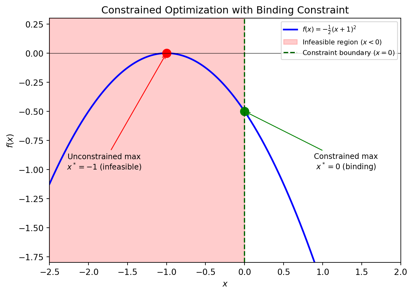
Example 1
\[ \begin{aligned} &\max \quad -\frac{1}{2}(x+1)^2\\ & \,\text{s.t.}\,\quad x \ge 0 \end{aligned} \]
The Lagrangian is:
\[ \mathcal{L} = -\frac{1}{2} (x+1)^2 + \mu x \]
FONC:
\[ [x]: \quad -(x+1) + \mu = 0, \quad \mu \ge 0 \]
So \((x+1) = \mu\) and \(\mu x = 0\) (either \(x=0\) or \(\mu=0\)).
Solution:
- If \(\mu=0 \Rightarrow x=-1\), contradicting the constraint \(x \ge 0\)
- Therefore \(\mu>0\) and \(x=0\)
- Thus \(\mu = 0 + 1 = 1\)
Shorthand: \(-(x+1) \le 0\), \(=0\) if \(x>0\)
Example 2
\[ \begin{aligned} &\max \quad f(x)\\ & \,\text{s.t.}\,\quad x \le m \end{aligned} \]
First, reorder the constraint: \(x - m \le 0 \Rightarrow m - x \ge 0\).
The Lagrangian is:
\[ \mathcal{L} = f(x) + \lambda(m-x) \]
FONC:
\[ \begin{aligned} [x]: \quad f'(x) - \lambda &= 0 \\ \lambda(m-x) &= 0, \quad \lambda \ge 0 \end{aligned} \]
The Kuhn-Tucker conditions are:
- If \(\lambda > 0 \Rightarrow m-x=0 \Rightarrow x=m\) (binding)
- If \(\lambda = 0 \Rightarrow f'(x)=0\) (nonbinding)
Linear Objectives Hit Corners
Consider for some \(a \in {\mathbb{R}}\):
\[ \begin{aligned} &\min \quad a x\\ & \,\text{s.t.}\,\quad x \geq 1 \end{aligned} \]
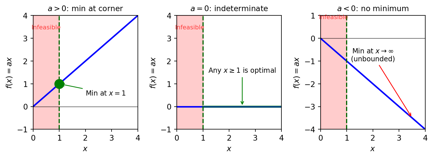
The cases:
- \(a > 0\): min is at \(x = 1\) (constraint binds)
- \(a = 0\): min is indeterminate (any \(x \geq 1\) works)
- \(a < 0\): min is at \(x = \infty\) (doesn’t exist, problem is unbounded)
Probability
Discrete Random Variables
A random variable is a number whose value depends upon the outcome of a random experiment. Mathematically, a random variable \(X\) is a real-valued function on \(S\), the space of outcomes:
\[ X: S \rightarrow {\mathbb{R}} \]
A discrete random variable \(X\) has finite or countably many values \(x_s\) for \(s = 1, 2, \ldots\)
The probabilities \({\mathbb{P}_{}\left( {X = x_s} \right)}\) for \(s = 1, 2, \ldots\) are called the probability mass function of \(X\), with properties:
- For all \(s\): \({\mathbb{P}_{}\left( {X = x_s} \right)} \geq 0\)
- For any \(B\subseteq S\): \({\mathbb{P}_{}\left( {X \in B} \right)} = \sum_{x_s \in B} {\mathbb{P}_{}\left( {X = x_s} \right)}\)
- \(\sum_s {\mathbb{P}_{}\left( {X = x_s} \right)} = 1\)
The expectation of \(X\) is:
\[ {\mathbb{E}_{{}}\left[ {X} \right]} = \sum_s x_s {\mathbb{P}_{}\left( {X = x_s} \right)} \]
Expectations and Vectors
Assume there are \(n\) states \(x_1, \ldots, x_n\). Define the values vector:
\[ x \equiv \begin{bmatrix} x_1 \\ x_2 \\ \vdots \\ x_n\end{bmatrix} \]
And the probability vector \(\phi \in {\mathbb{R}}^n\):
\[ \phi \equiv \begin{bmatrix} {\mathbb{P}_{}\left( {X = x_1} \right)}\\ {\mathbb{P}_{}\left( {X = x_2} \right)} \\ \vdots \\ {\mathbb{P}_{}\left( {X = x_n} \right)}\end{bmatrix} \]
Then the expectation can be written as a dot product:
\[ {\mathbb{E}_{{}}\left[ {X} \right]} = \sum_{i=1}^{n} \phi_i x_i = \phi \cdot x \]
Example: Probability of unemployment is \(\phi_1 = 0.1\) with income \(x_1 = \$15{,}000\); probability of employment is \(\phi_2 = 0.9\) with income \(x_2 = \$40{,}000\). Expected income:
\[ {\mathbb{E}_{{}}\left[ {X} \right]} = (0.1 \times 15{,}000) + (0.9 \times 40{,}000) = \$37{,}500 \]
More generally, this extends to functions of random variables: \({\mathbb{E}_{{}}\left[ {X^2} \right]} = \phi \cdot x^2\).
Joint Distributions
For discrete random variables \(X\) and \(Y\), the joint probability distribution is:
\[ {\mathbb{P}_{}\left( {X = x_i \text{ and } Y = y_j} \right)} \]
such that \(\sum_i\sum_j {\mathbb{P}_{}\left( {X = x_i \text{ and } Y = y_j} \right)} = 1\).
Marginal Probability
The distribution of one random variable, ignoring the other:
\[ {\mathbb{P}_{}\left( {X = x_i} \right)} = \sum_j {\mathbb{P}_{}\left( {X = x_i \text{ and } Y = y_j} \right)} \]
Conditional Probability
The distribution of one random variable given the other has occurred:
\[ {\mathbb{P}\left( {X = x_i}\left| {Y=y_j} \right. \right)} = \frac{{\mathbb{P}_{}\left( {X = x_i \text{ and } Y = y_j} \right)}}{{\mathbb{P}_{}\left( {Y = y_j} \right)}} = \frac{{\mathbb{P}_{}\left( {X = x_i \text{ and } Y = y_j} \right)}}{\sum_k {\mathbb{P}_{}\left( {X = x_k \text{ and } Y = y_j} \right)}} \]
Conditional Expectation
When one event is known, the expectation over the other:
\[ {\mathbb{E}_{{}}\left[ {X \mid Y = y_j} \right]} = \sum_i x_i {\mathbb{P}\left( {X = x_i}\left| {Y = y_j} \right. \right)} \]
This is especially useful for agents making forecasts of the future given knowledge of events today.
Statistical Independence
Events \(X\) and \(Y\) are statistically independent if:
\[ {\mathbb{P}_{}\left( {X = x_i \text{ and } Y = y_j} \right)} = {\mathbb{P}_{}\left( {X = x_i} \right)}{\mathbb{P}_{}\left( {Y = y_j} \right)} \]
If \({\mathbb{P}_{}\left( {Y = y_j} \right)} > 0\), independence implies \({\mathbb{P}\left( {X = x_i}\left| {Y=y_j} \right. \right)} = {\mathbb{P}_{}\left( {X = x_i} \right)}\).