Incomplete Markets and Dynamic Programming
Honours Intermediate Macro
Permanent income with no-borrowing constraints, Lagrangian methods for inequality constraints, and dynamic programming
Basic Setup
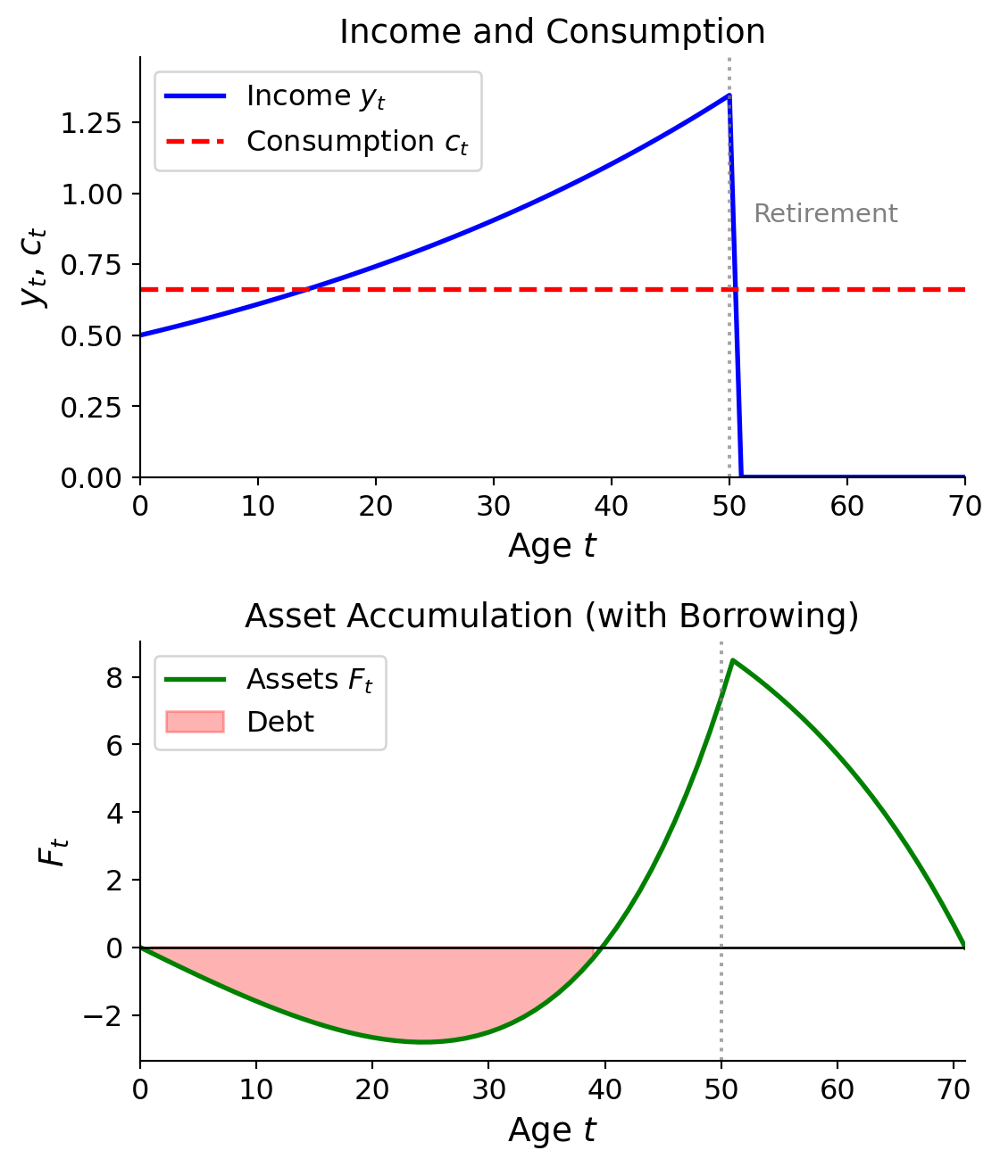
As shown in Figure 1, with growing income and retirement, assets may become negative early in the lifecycle (borrowing against future income). Note that debt does not bottom out when \(y_t = c_t\)—at that point, interest on existing debt still causes debt to grow. Debt stops increasing only when savings cover the interest burden: \(y_t > c_t + \frac{-r}{1+r}F_t\), i.e., when income exceeds consumption by enough to offset interest payments on existing debt.
What happens if we add a no-borrowing constraint?
Adding Constraints to the PIH
\[ \max_{\{c_t, F_{t+1}\}} \sum_{t=0}^{\infty} \beta^t u(c_t) \]
subject to:
\[ \begin{aligned} F_{t+1} &= R(F_t + y_t - c_t) \\ \lim_{T \to \infty} \beta^{T+1} F_{T+1} &\geq 0 \quad \text{(No Ponzi)} \\ F_{t+1} &\geq 0 \quad \text{(No borrowing!)} \\ c_t &\geq 0 \end{aligned} \]
where \(F_0\) is given, \(\beta < 1\), \(R > 1\). Assume \(\lim_{c \to 0} u'(c) = \infty\) (called an “Inada Condition”).
Setting Up the Lagrangian
\[ \mathcal{L} = \sum_{t=0}^{\infty} \beta^t \left( u(c_t) + \lambda_t [R(F_t + y_t - c_t) - F_{t+1}] + \nu_{t+1} \cdot F_{t+1} + \alpha_t \cdot c_t \right) \]
where:
- \(\lambda_t\) is the Lagrange multiplier on the intertemporal budget constraint
- \(\nu_{t+1}\) is the Lagrange multiplier on \(F_{t+1} \geq 0\)
- \(\alpha_t\) is the Lagrange multiplier on \(c_t \geq 0\)
First Order Necessary Conditions:
\[ \begin{aligned} [c_t]: \quad & \beta^t u'(c_t) - \beta^t \lambda_t R + \beta^t \alpha_t = 0, \quad \forall t \geq 0 \\ [F_{t+1}]: \quad & -\lambda_t + \nu_{t+1} + \beta \lambda_{t+1} R = 0, \quad \forall t \geq 0 \end{aligned} \tag{1}\]
Complementary Slackness Conditions:
\[ \begin{aligned} \nu_{t+1} &\geq 0, \quad \alpha_t \geq 0 \\ \nu_{t+1} F_{t+1} &= 0, \quad \alpha_t c_t = 0 \end{aligned} \]
Deriving the Euler Equation
Reorganizing the FOC for \(c_t\):
\[ u'(c_t) + \alpha_t = \lambda_t R, \quad \text{with } \alpha_t \geq 0 \implies u'(c_t) \leq \lambda_t R, \text{ with equality if } \alpha_t = 0 \]
From complementary slackness, either \(\alpha_t = 0\) or \(c_t = 0\). If \(c_t = 0\), the Inada condition implies \(u'(0) = \infty\), which contradicts \(u'(c_t) \leq \lambda_t R\). Therefore \(\alpha_t = 0\) and \(c_t > 0\), giving us:
\[ \boxed{u'(c_t) = \lambda_t \cdot R} \tag{2}\]
Reorganizing the FOC for \(F_{t+1}\) and multiplying by \(R\):
\[ \beta R^2 \lambda_{t+1} - R \lambda_t + R \nu_{t+1} = 0 \]
Using Equation 2 to substitute:
\[ \beta R u'(c_{t+1}) + R \nu_{t+1} = u'(c_t) \]
Since \(\nu_{t+1} \geq 0\), with equality when \(F_{t+1} > 0\):
\[ \beta R u'(c_{t+1}) \leq u'(c_t), \quad \text{with equality if } F_{t+1} > 0, \quad \forall t \geq 0 \]
Note that if \(F_{t+1} = 0\) and \(\nu_{t+1} > 0\), then from the budget constraint:
\[ 0 = R(F_t + y_t - c_t) \implies c_t = F_t + y_t \quad \text{(consumes all income and savings)} \]
Summary: Euler Equation with No-Borrowing Constraints
\[ \boxed{ \begin{aligned} &u'(c_t) = \beta R u'(c_{t+1}); \quad \text{or} \\ &u'(c_t) > \beta R u'(c_{t+1}) \quad \textbf{and} \quad c_t = F_t + y_t \end{aligned} } \]
Examples with Log Utility
Assume \(u(c) = \log(c) \implies u'(c) = \frac{1}{c}\) and \(\beta R = 1\).
Then:
\[ \begin{aligned} &\frac{1}{c_t} = \frac{1}{c_{t+1}} \implies c_{t+1} = c_t; \quad \text{or} \\ &\frac{1}{c_t} > \frac{1}{c_{t+1}} \implies c_{t+1} > c_t \quad \textbf{and} \quad c_t = F_t + y_t \end{aligned} \]
Example 1: Growing Income (Always Constrained)
Let \(y_{t+1} = \delta y_t \implies y_t = \delta^t y_0\) with \(\delta > 1\) and \(F_0 = 0\).
Solution: Guess always constrained, then verify.
\[ c_t = y_t, \quad F_t = 0, \quad \forall t \]
So the person is always borrowing constrained.
Verification: \(y_t > y_{t-1} \implies c_t > c_{t-1}\), \(\forall t\); and \(F_t = 0 \implies c_t = y_t\).
Example 2: Decreasing Income (Never Constrained)
Let \(0 < \delta < 1\), \(y_t = \delta^t y_0\), \(F_0 = 0\).
Solution: Guess unconstrained, then verify.
Guess \(c_t = \bar{c}\), using the unconstrained formula with \(F_0 = 0\):
\[ \bar{c} = (1 - \beta) y_0 \sum_{t=0}^{\infty} \delta^t \beta^t = (1 - \beta) \frac{y_0}{1 - \beta \delta} \]
\[ \boxed{\bar{c} = (1 - \beta) \frac{y_0}{1 - \beta \delta}} \]
Assets evolve according to:
\[ F_{t+1} = R(F_t + y_t - \bar{c}) \]
Note: \(c_0 = \frac{1-\beta}{1-\beta\delta} y_0 < \frac{1-\beta}{1-\beta} y_0 = y_0 \implies y_0 - c_0 > 0\), so the agent saves, not borrows.
In the limit as \(t \to \infty\), \(y_t \to 0\) but \(c_t = \bar{c}\). Looking for a steady state in the budget:
\[ \bar{F} = R(\bar{F} + 0 - \bar{c}) \implies R \bar{c} = (R-1) \bar{F} \]
Since \(R = 1 + r\):
\[ \bar{c} = \frac{R-1}{R} \bar{F} = \underbrace{\frac{r}{1+r}}_{\text{annuity value}} \bar{F} \]
So the agent eventually lives off the annuity value of savings. (Also \(\frac{r}{1+r} = 1 - \beta\) if \(\beta \equiv \frac{1}{1+r}\).)
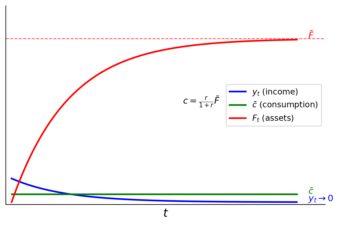
See Figure 2 for the asymptotic behavior with decreasing income.
Welfare Cost of No-Borrowing
We now analyze the welfare cost of borrowing constraints more generally. This analysis follows Ljungqvist and Sargent (2018).
Setup:
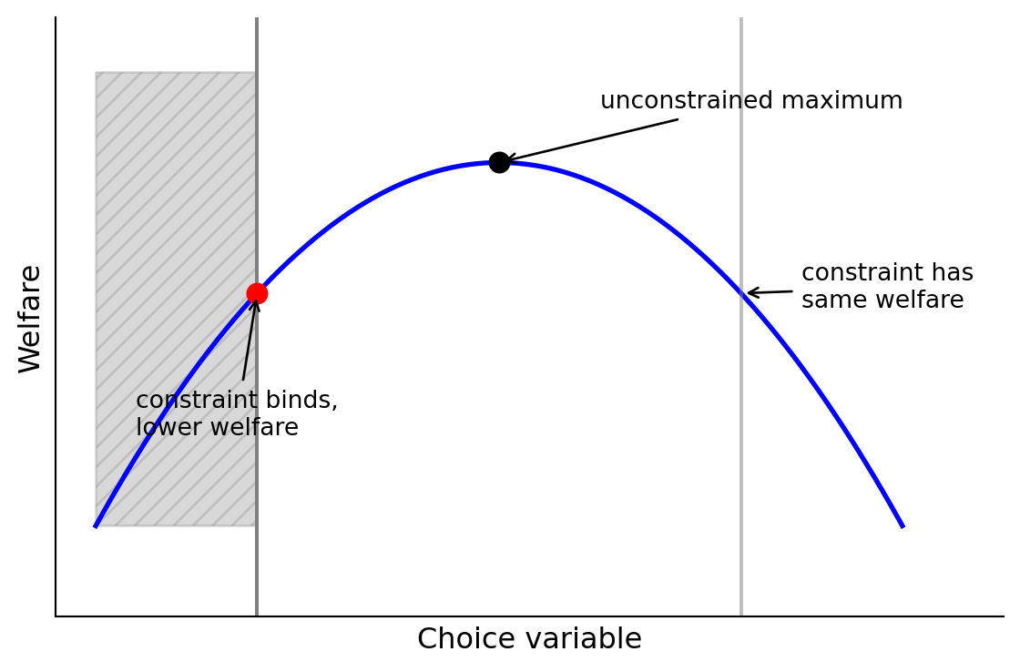
- Given a feasible \(\{c_t\}\), the lifetime utility of an agent is \(U = \sum_{t=0}^{\infty} \beta^t u(c_t)\). This is their welfare, their objective function.
- In general, adding constraints to the set of feasible \(\{c_t\}\) weakly decreases welfare, as shown in Figure 3.
Unconstrained Solution (\(T = \infty\))
Now consider a case where the agent wants to borrow: income grows faster than the optimal consumption path. Assume \(1 \leq \beta R \leq \delta\) (so income growth \(\delta\) exceeds or equals consumption growth \(\beta R\)), \(u(c) = \log(c)\), \(F_0 = 0\), subject to \(\lim_{T \to \infty} F_{T+1} \beta^T \geq 0\) (no Ponzi scheme).
Euler Equation:
\[ u'(c_t) = \beta R u'(c_{t+1}) \implies c_{t+1} = \beta R c_t \implies c_t = (\beta R)^t c_0 \]
Lifetime Budget:
\[ 0 = \sum_{j=0}^{\infty} R^{-j}(c_{t+j} - y_{t+j}) \]
\[ \sum_{t=0}^{\infty} R^{-t} \beta^t R^t c_0 = \sum_{t=0}^{\infty} R^{-t} \delta^t y_0 \implies \underbrace{\frac{c_0}{1-\beta}}_{\text{PV of consumption}} = \underbrace{\frac{y_0}{1 - \delta/R}}_{\text{PV of income}} \]
\[ \implies c_0 = (1-\beta) \frac{y_0}{1 - \delta/R} \]
Consumer’s Lifetime Utility:
\[ \begin{aligned} U &= \sum_{t=0}^{\infty} \beta^t \log(c_t) = \sum_{t=0}^{\infty} \beta^t \log\left( (\beta R)^t \cdot \frac{1-\beta}{1-\delta/R} y_0 \right) \\ &= \sum_{t=0}^{\infty} \beta^t \left[ \log(y_0) + \log\left(\frac{1-\beta}{1-\delta/R}\right) + t \log(\beta R) \right] \\ &= \frac{\log y_0 + \log(1-\beta) - \log(1-\delta/R)}{1-\beta} + \log(\beta R) \sum_{t=0}^{\infty} t \beta^t \end{aligned} \]
Using \(\sum_{t=0}^{\infty} t \beta^t = \frac{\beta}{(1-\beta)^2}\):
\[ \boxed{U = \frac{1}{1-\beta}\left[\log(y_0) + \log(1-\beta) - \log(1-\delta/R)\right] + \log(\beta R) \frac{\beta}{(1-\beta)^2}} \]
No-Borrowing Solution (\(T = \infty\))
Same assumptions but with \(F_{t+1} \geq 0\).
Since the agent wants to borrow but cannot, they are always constrained (as in Example 1). The agent consumes all income each period: \(c_t = y_t = y_0 \delta^t\).
\[ \begin{aligned} U^{NB} &= \sum_{t=0}^{\infty} \beta^t \log(y_0 \delta^t) = \sum_{t=0}^{\infty} \beta^t \left[ \log(y_0) + t \log(\delta) \right] \\ &= \frac{\log(y_0)}{1-\beta} + \log(\delta) \sum_{t=0}^{\infty} t \beta^t \\ &= \frac{\log(y_0)}{1-\beta} + \log(\delta) \frac{\beta}{(1-\beta)^2} \neq U \end{aligned} \]
The welfare loss from the no-borrowing constraint is \(U - U^{NB}\).
Dynamic Programming Approach
Suppose \(c_t = c_0 \delta^t\) for \(t \geq 0\). We want to evaluate:
\[ V(c_0) = \sum_{t=0}^{\infty} \beta^t \log(c_t) \]
Note:
\[ V(c_0) = \log(c_0) + \beta \sum_{j=0}^{\infty} \beta^j \log(c_{1+j}) = \log(c_0) + \beta V(c_1) \]
where \(c_1 = \delta c_0\). This is Markov!
Bellman Equation:
\[ V(c) = \log(c) + \beta V(\delta c) \]
We want to find the \(V(c)\) function, then evaluate at \(c_0\).
Solving by Undetermined Coefficients
Guess: \(V(c) = k_0 + k_1 \log(c)\), where \(k_0, k_1\) are undetermined coefficients.
Plug in:
\[ \begin{aligned} k_0 + k_1 \log(c) &= \log(c) + \beta [k_0 + k_1 \log(\delta c)] \\ &= \log(c) + \beta k_0 + \beta k_1 \log(\delta) + \beta k_1 \log(c) \\ &= \underbrace{[1 + \beta k_1]}_{= k_1} \log(c) + \underbrace{[\beta k_0 + \beta k_1 \log(\delta)]}_{= k_0} \end{aligned} \]
Matching coefficients:
\[ \begin{aligned} k_1 &= 1 + \beta k_1 \implies k_1 = \frac{1}{1-\beta} \\ k_0 &= \beta k_0 + \beta k_1 \log(\delta) = \beta k_0 + \beta \frac{\log(\delta)}{1-\beta} \implies k_0 = \frac{\beta}{(1-\beta)^2} \log(\delta) \end{aligned} \]
Therefore:
\[ \boxed{V(c) = \frac{1}{1-\beta} \log(c) + \frac{\beta}{(1-\beta)^2} \log(\delta)} \]
This agrees with our earlier solution for welfare.
References
Ljungqvist, Lars, and Thomas J. Sargent. 2018. Recursive Macroeconomic Theory. 4th ed. MIT Press.