Linear Difference Equations and Asset Pricing
Honours Intermediate Macro
Solving difference equations, rational bubbles, and linear state space models for asset pricing
Solutions (and Uniqueness) of Difference Equations
From the previous lecture notes, pricing a sequence \(\left\{{y_{t+j}}\right\}\) of payoffs:
\[ P_t = \sum_{j=0}^{\infty} \beta^j y_{t+j} \quad \text{at time } t \text{ (Sequential formulation)} \]
Can be written:
\[ P_t = y_t + \beta P_{t+1} \]
Solving with Guess and Verify
How can we solve a difference equation?
Example: \(y_t=\bar{y}\)
\[ P_t = \bar{y} + \beta P_{t+1} \tag{1}\]
A Guess: \(P_t=\bar{P}\), independent of \(t\). Plug in Equation 1:
\[ \bar{P} = \bar{y} + \beta \bar{P} \quad \Rightarrow \quad \bar{P} = \frac{\bar{y}}{1-\beta}, \text{ consistent with } P=\sum_{t=0}^{\infty} \beta^t y_t \]
Role of \(|\beta|<1\):
- Keep from “exploding”: stability
- Will have equivalent condition for more complicated difference equations
Rational Bubbles
Let \(y_t=\bar{y}\) for all \(t\).
Fundamental value:
\[ P_t = \sum_{j=0}^{\infty} \beta^j \bar{y} = \frac{\bar{y}}{1-\beta} \quad \text{(unique)} \]
Remember that this solves the recursive problem as well:
\[ \frac{\bar{y}}{1-\beta} = \bar{y} + \beta \left(\frac{\bar{y}}{1-\beta}\right) \Rightarrow \text{true!} \]
Is \(P_t = \dfrac{\bar{y}}{1-\beta}\) the unique solution to \(P_t = \bar{y} +\beta P_{t+1}\)? No! Like the undetermined coefficient in differential equations.
Example:
\[ P_t = \underbrace{\dfrac{\bar{y}}{1-\beta}}_{\text{fundamental value}} + \underbrace{c \beta^{-t}}_{\text{bubble term}} \quad \text{for any } c \]
Check: \(P_t = \bar{y} + \beta P_{t+1}\)
\[ \frac{\bar{y}}{1-\beta} + c\beta^{-t} = \bar{y} + \beta \left[ \frac{\bar{y}}{1-\beta} + c \beta^{-(t+1)} \right] = \bar{y} + \left(\frac{\beta}{1-\beta}\right)\bar{y} + c\beta^{-t} = \frac{\bar{y}}{1-\beta} + c\beta^{-t} \]
So it fulfills the difference equation for any \(c,t\), etc. Rational as every agent in the economy would agree on the price, no one needs to be tricked or making a pricing mistake, and there is no arbitrage. An example of a self-fulfilling equilibrium.
Size of the “Rational Bubble”
\[ \underbrace{P_0 - P_{fund}}_{\text{difference from fundamental}} = \frac{\bar{y}}{1-\beta} - \frac{\bar{y}}{1-\beta} + c \beta^0 = c \]
Expectations:
- Prices rise because they are expected to rise.
- Self-fulfilling. Will depend on coordination of expectations.
- Is Fiat money a bubble?
Extending our Asset Pricing Model
We will generalize our results to include systems of equations, with dynamics.
Recall: Properties
- Dividend stream \(y_t\)
- Discount factor \(\beta\)
- Present discounted value = price: \(P = \sum_{t=0}^{\infty} \beta^t y_t\), and if \(y_t = \bar{y}\), \(P=\bar{y}(1-\beta)^{-1}\)
- How to model the evolution of \(y_t\)?
- Will use systems of linear difference equations in an underlying state \(x_t\)
- Example: dividends are a linear function of evolving aggregate and idiosyncratic variables
Recall: Recursive Formulation: \(P_t = y_t + \beta P_{t+1}\)
Applying to Dynamics
- Let \(x_t\) be an \(n\)-dimensional vector of states.
- Let \(A, G\) be matrices.
- Stack first order difference equations, giving another canonical form:
\[ \begin{aligned} x_{t+1} &= A \cdot x_t & \text{($A$ is $n \times n$ matrix, $x_t$ is $n \times 1$ vector)}\\ y_t &= G \cdot x_t & \text{($G$ is $1 \times n$ vector, $y_t$ is a scalar, i.e. $1 \times 1$)} \end{aligned} \]
- “\(A\)” gives evolution of the state, given \(x_0\)
- “\(G\)” gives observation of the state
- “Finding the state is an art”
Example:
- Asset payoff follows difference equation (not first order!):
\[ y_{t+1} = \rho_1 y_t + \rho_2 y_{t-1} \]
- What is the value of this asset at time \(t\)?
State:
Guess: \(x_t \equiv \begin{bmatrix} y_t \\ y_{t-1} \end{bmatrix}\), a \(2 \times 1\) vector.
What is the difference equation for \(x_t\)?
\[ \underbrace{\begin{bmatrix} y_{t+1} \\ y_t \end{bmatrix}}_{x_{t+1}} = \underbrace{\begin{bmatrix} \rho_1 & \rho_2 \\ 1 & 0 \end{bmatrix}}_{A} \underbrace{\begin{bmatrix} y_{t} \\ y_{t-1} \end{bmatrix}}_{x_t} \]
And observation:
\[ y_t = \underbrace{\begin{bmatrix} 1 & 0 \end{bmatrix}}_{G} \underbrace{\begin{bmatrix} y_t \\ y_{t-1} \end{bmatrix}}_{x_t} \]
Therefore, the set of difference equations in our canonical form are:
\[ \begin{aligned} x_{t+1} &= Ax_t\\ y_t &= Gx_t \end{aligned} \]
Price is:
\[ P_t = \sum_{j=0}^{\infty} \beta^j y_{t+j} = \sum_{j=0}^{\infty} \beta^j G \cdot x_{t+j} \]
If \(x_{t+1} = A\cdot x_t\), then \(x_{t+2} = A \cdot (A x_t) = A^2 x_t\), and \(x_{t+j} = A^j x_t\)
\[ \Rightarrow P_t = \sum_{j=0}^{\infty} \beta^j G \cdot A^j \cdot x_t = G \cdot \left[ \sum_{j=0}^{\infty} \left(\beta A\right)^j \right] x_t \]
Remember that if \(\lambda\) is scalar: \(\sum_{j=0}^{\infty} \left(\beta \lambda\right)^j = \left(1-\beta\lambda\right)^{-1} = \frac{1}{1-\beta \lambda}\).
With matrices and inverses, this is similar: \(\sum_{j=0}^{\infty} \beta^j A^j = \left(I - \beta A\right)^{-1}\),
where the matrices’ dimensions are: \(A : n \times n\), \(I = n \times n\) identity, \((I-\beta A)^{-1} : n \times n\)
\[ \boxed{P_t = G \left(I-\beta A\right)^{-1} x_t} \quad (\text{very important, memorize!}) \]
- Asset pricing formula for first-order linear difference equations.
- Summary of sizes:
- \(P_t\): \(1 \times 1\) scalar
- \(G\): \(1 \times n\) vector
- \(A\): \(n \times n\) matrix
- \(I\): \(n \times n\) identity matrix
- \(\beta\): \(1 \times 1\) scalar
- \(x_t\): \(n \times 1\) state vector
Stability
- Recall in the example with \(x_t = \lambda^t\) that \(|\beta \lambda| < 1\) for the series to converge.
- For matrix equations, need a similar condition where eigenvalues of \(\beta A\) are all \(<1\), or \(\max | \text{eig}(A) | < \frac{1}{\beta}\)
- Can use software to check the eigenvalues.
Appendices
Connection to Differential Equations
Difference equations are just differential equations in discrete time.
- Let \(y(t)\) be the flow dividends, a function of \(t\).
- Let \(r\) be the instantaneous interest rate.
- Let the length of a period be \(\Delta\), and take the limit as it goes to 0.
- Dividends over \(\Delta\) period \(\approx \Delta y(t) \equiv y_t(\Delta)\)
- Discounting over \(\Delta\) period \(\approx 1- \Delta r \equiv \beta(\Delta)\)
The difference equation is: \(P_t = y_t + \beta P_{t+1}\).
Using the above: Let function \(p(t)\) be the price of asset:
\[ p(t) = \Delta \cdot y(t) + (1-\Delta r) \cdot p(t+\Delta) \]
Rearrange:
\[ \Delta r \cdot p(t+\Delta) = \Delta \cdot y(t) + p(t+\Delta) - p(t) \]
\[ \Rightarrow r p(t+\Delta) = y(t) + \frac{p(t+\Delta) - p(t)}{\Delta} \]
Take limit as \(\Delta \rightarrow 0\), i.e. discrete \(\rightarrow\) continuous \(t\)
\[ {\boldsymbol{\partial}_{}}p(t) = \frac{p(t+\Delta) - p(t)}{\Delta} \quad \text{(definition of a derivative)} \]
where \({\boldsymbol{\partial}_{}}p(t) = \dfrac{d}{dt}p(t)\)
\[ \Rightarrow \underbrace{r p(t)}_{\text{opportunity cost of buying a unit of the asset}} = \underbrace{y(t)}_{\text{flow dividends}} + \underbrace{{\boldsymbol{\partial}_{}}p(t)}_{\text{capital gains}} \]
- Consider this pricing equation and arbitrage:
- What if \(r p(t) < y(t) + {\boldsymbol{\partial}_{}}p(t)\) instead of being an equation?
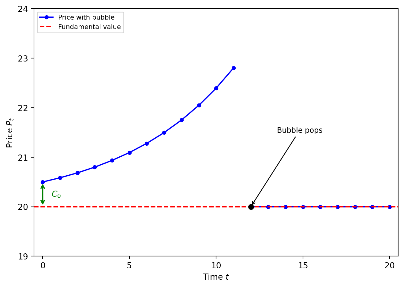
Popping Bubbles
In our discrete time model, keep \(y_t=\bar{y}\) deterministic for simplicity:
- Let the bubble term have a chance of popping each period.
- Therefore, prices are a random variable.
- Linear asset pricing if random:
\[ P_t = y_t + \beta {\mathbb{E}_{{t}}\left[ {P_{t+1}} \right]} \quad \text{(Expected value of $P_{t+1}$ given information at $t$)} \]
Bubble Evolution
\[ \text{Let } C_{t+1} = \begin{cases} \frac{1}{\lambda} C_t & \text{with prob. } \lambda \in (0,1) \\ 0 & \text{with prob. } 1-\lambda \end{cases} \]
i.e., \(C_t\) multiplied by \(\frac{1}{\lambda}\) each time until bubble breaks. Then \(C_t = 0\) for all \(t\).
Note:
\[ {\mathbb{E}_{{t}}\left[ {C_{t+1}} \right]} = \lambda \left(\frac{1}{\lambda} C_t\right) + (1-\lambda)\cdot 0 = C_t \]
If \({\mathbb{E}_{{t}}\left[ {y_{t+1}} \right]}=y_t\), then this term is called a martingale.
Price Level
We can check that for any \(C_0\):
\[ P_{t} = \begin{cases} \frac{\bar{y}}{1-\beta} + \left(\beta \lambda\right)^{-t}\cdot C_0 & \text{if bubble hasn't popped} \\ \frac{\bar{y}}{1-\beta} & \text{after bubble pops} \end{cases} \]