<torch._C.Generator at 0x7f3474270c10>Transformers and Attention
Machine Learning Fundamentals for Economists
Overview
Summary
- Describe “attention” with function approximation and relate to kernels and similarity
- Describe transformers, the architecture that makes LLMs possible
- Give intuition on how/when transformers can work
- Describe it more generally as a tool for sequential and set-based data (e.g., graphs, images)
References
- The transformer model is complicated and uses some building blocks we haven’t formally introduced
- These notes are a bare-bones introduction.
- Melissa Dell’s Course has plenty of details:
- ProbML Book 1 and ProbML Book 2
Packages
Attention
Reminder: Kernel Regression
- Recall in the Kernels/GP lecture we discussed how we can define a kernel to do pairwise comparisons of two inputs from a set of data \(X = \{x_1, x_2, \ldots, x_n\}\) with outputs \(Y = \{y_1, y_2, \ldots, y_n\}\).
- \(\mathcal{K}(x_i, x_j)\) is a measure of similarity between \(x_i\) and \(x_j\).
- Then, for a new \(x\), we could define a vector of similarity scores, \(\alpha(x) \equiv [\mathcal{K}(x, x_i)]_{i=1}^n\)
- And “predict” a \(y(x)\) as a weighted sum of the \(y_i\)’s \[ y(x) \approx \sum_{i=1}^n \mathcal{K}(x, x_i) y_i = \alpha(x) \cdot Y \]
- Non-parametric, with potentially infinite-dimensional feature spaces
Attention as a Fuzzy Look-up Table
- We can think of kernel regression as a non-parametric model of attention (see ProbML Book 1 Section 15.4.2)
- A fuzzy look-up table with three ingredients:
- Query \(x\): the input you want to look up
- Keys \(x_1, \ldots, x_n\): the stored entries you compare against
- Values \(y_1, \ldots, y_n\): the output associated with each key
- The look-up is “fuzzy” because instead of returning a single exact match:
- Score each key by similarity: \(\alpha_i(x) = x \cdot x_i\) (dot product)
- Normalize to probabilities: \(\alpha_i(x) / \sum_{i'} \alpha_{i'}(x)\)
- Return the weighted average of values: \(\sum_i \alpha_i(x)\, y_i\)
Parametric Version
- Taking that inspiration, we want to define a version of this which is parametric (i.e., it will not require saving all the data in memory) and is differentiable
- To be parametric, replace the fixed kernels based on the data with a parametric form as a learned embedding
- In order to be differentiable, we want to replace a fixed lookup table with a probabilistic one
- Kernel Regressions evaluated on new \(\{x_1, \ldots, x_n\}\) required pairwise comparison within that set, and across all previous data.
- Parametric versions can just compare the new \(x\) to each other pairwise using the embedding
- See ProbML Book 1 Section 15.4 and ProbML Book 2 Section 16.2.7 for more
From Token IDs to Vectors
- Attention operates on continuous vectors, but LLM inputs are discrete token IDs \(c \in \{1,\ldots,C\}\) where \(C\) is the vocabulary size
- Represent each token as a one-hot (i.e., dummy variable) vector \(e_c \in \{0,1\}^{C}\), with a \(1\) in position \(c\)
- A learned token-embedding matrix \(W_E \in {\mathbb{R}}^{C \times h}\) maps this to a dense vector \[
x = e_c^\top W_E \in {\mathbb{R}}^h
\]
- This is just a lookup of row \(c\) of \(W_E\) — but writing it as a matrix multiply makes it differentiable and end-to-end trainable
- \(W_E\) is learned jointly with all other parameters (attention weights, etc.)
- Positional encodings are added to \(x\) so the model knows token order (discussed later)
- Recall from the Embeddings lecture: tokenizers split text → token IDs; this matrix turns those IDs into the vectors that attention consumes
Mapping to an Embedding Space
- Starting from token embeddings \(x \in {\mathbb{R}}^h\), learn three linear projections:
- Query: \(q = x W_Q\) for \(W_Q \in {\mathbb{R}}^{h \times d}\)
- Key: \(k = x W_K\) for \(W_K \in {\mathbb{R}}^{h \times d}\)
- Value: \(v = x W_V\) for \(W_V \in {\mathbb{R}}^{h \times v}\)
- Queries and keys live in the same \(d\)-dimensional space (so their dot product is defined); values can have a different dimension \(v\)
- For \(n\) input tokens, stack rows into matrices \(Q \in {\mathbb{R}}^{n \times d}\), \(K \in {\mathbb{R}}^{n \times d}\), and \(V \in {\mathbb{R}}^{n \times v}\)
Attention for a Single “Query”
- Given a \(q\), the attention is \[ \begin{aligned} \text{Attn}(q, K, V) &\equiv \sum_{i=1}^n \alpha_i(q, K)\cdot V_i\\ \alpha_i(q, K) &\equiv \frac{\exp(a(q, K_i))}{\sum_{j=1}^n \exp(a(q, K_j))} && \small\text{(attention weight on key } i\text{)}\\ a(q, k) &\equiv q \cdot k/\sqrt{d} && \small\text{(similarity score)} \end{aligned} \]
- The output is a weighted combination of values: each value \(V_i\) contributes in proportion to how well its key matches the query
- The weights \(\alpha_i\) are a softmax over similarity scores — so they are non-negative and sum to 1
Attention Layer
- Typically we are calculating the attention for a sequence of \(n\) embedded inputs
- Use \(W_Q\) to embed inputs, \(Q \in {\mathbb{R}}^{n \times d}\), then \[
Z = \text{Attn}(Q, K, V) = \mathrm{softmax}\left(\frac{Q K^{\top}}{\sqrt{d}}\right)V \in {\mathbb{R}}^{n \times v}
\]
- The parameters to “learn” are just the embeddings, \(W_Q, W_K\) and potentially \(W_V\)
- Why \(1/\sqrt{d}\)? If entries of \(q, k\) have unit variance, \(q \cdot k\) has variance \(\approx d\)
- Without rescaling, softmax collapses toward putting all weight on one key — deterministic rather than fuzzy lookup
- Mechanically changes the “temperature” of softmax. See the Embeddings lecture
Scaled Dot-Product Attention in Code
C, d, n = 3, 4, 3  # vocab size, embedding dim, sequence length

# One-hot encoding → embedding
token_ids = torch.tensor([0, 2, 1])
one_hot = F.one_hot(token_ids, num_classes=C).float()
W_E = torch.randn(C, d)
X = one_hot @ W_E  # (n, d) embedded tokens

# Learned projection matrices
W_Q = torch.randn(d, d)
W_K = torch.randn(d, d)
W_V = torch.randn(d, d)

Q = X @ W_Q # broadcasts to all tokens
K = X @ W_K
V = X @ W_V

# Scaled dot-product attention (manual)
scores = (Q @ K.T) / d**0.5
weights = torch.softmax(scores, dim=-1)
output = weights @ V

print("Attention weights (each row sums to 1):")
print(weights.detach().numpy().round(3))
print("Output:")
print(output.detach().numpy().round(3))
Attention weights (each row sums to 1):
[[0.283 0.313 0.404]
[0.142 0.172 0.687]
[0.756 0.242 0.001]]
Output:
[[-1.087  1.036 -1.564  0.502]
 [-1.771  1.595 -2.899  1.01 ]
[-0.184 0.118 0.385 -0.133]]PyTorch Built-in Attention
Multi-Head Attention
There will be different senses of similarity for the query, key, and value.
A powerful approach is to have multiple self-attention layers \(j=1,\ldots J\) \[ Z^j = \text{Attn}(X W_Q^j, X W_K^j, X W_V^j) \]
Then concatenate the \(Z^j\)’s along the feature dimension and project with embedding \(W_O\)
\[ \text{MultiHead}(X) = \text{Concat}(Z^1, \ldots, Z^J) \cdot W_O \]
- “Trainable” parameters are the \(W_Q^j, W_K^j, W_V^j, W_O\)
Multi-Head Attention in PyTorch
nn.MultiheadAttentionincludes the output projection \(W_O\) (out_proj)
# X persists from earlier: (n=3, d=4) embedded tokens
mha = nn.MultiheadAttention(embed_dim=d, num_heads=2, batch_first=True)

# Self-attention: all heads run in parallel on the same X
mha_output, mha_weights = mha(
    X.unsqueeze(0), X.unsqueeze(0), X.unsqueeze(0)
)

print("Attention weights (2 heads, averaged):")
print(mha_weights[0].detach().numpy().round(3))
print("\nOutput (n×d) — one row per token:")
print(mha_output[0].detach().numpy().round(3))
Attention weights (2 heads, averaged):
[[0.328 0.347 0.324]
[0.325 0.383 0.292]
[0.398 0.415 0.187]]
Output (n×d) — one row per token:
[[-0.311 0.217 -0.162 -0.223]
[-0.298 0.204 -0.149 -0.222]
[-0.381 0.261 -0.098 -0.273]]Multi-Head Attention in NNX
# NNX wraps jax.nn.dot_product_attention with learned projections
mha_nnx = nnx.MultiHeadAttention(
    num_heads=2, in_features=d, decode=False, rngs=nnx.Rngs(42)
)

# Self-attention: pass X once (key/value default to query)
X_jax = jnp.array(X.detach().numpy())
output_nnx = mha_nnx(X_jax[None, :, :])  # add batch dim

print("Output shape:", output_nnx.shape)
print(output_nnx[0].round(3))
Output shape: (1, 3, 4)
[[-0.45400003 -1.388 -0.75000006 -0.39100003]
[-0.45400003 -1.393 -0.734 -0.41900003]
[-0.393 -1.1960001 -0.698 -0.18100001]]Self-Attention
Interpretation
A standard, broad interpretation of attention for tokens
- The query contains what information a token is looking for
- The key contains what type of information a token provides
- The value contains what information is returned
Computational Cost of Attention
- The score matrix \(QK^\top \in {\mathbb{R}}^{n \times n}\) costs \(\mathrm{O}(n^2 d)\) compute and \(\mathrm{O}(n^2)\) memory
- Modern context windows reach \(n \approx 1{-}2\) million tokens
- Quadrupling the context length costs 16× in attention computation
- This quadratic cost is the binding constraint on context length
- Active research on reducing this cost:
- Sparse attention: attend only to local windows or selected tokens
- Linear attention: approximate softmax to avoid materializing \(n \times n\)
- FlashAttention: hardware-aware tiling that reduces memory I/O (exact, not approximate)
Self-Attention
- If the \(Q, K,\) and \(V\) come from the same data, then it is called self-attention
- Canonical example might be that \(X\) are embedded tokens of a sentence
- That is, if we have an \(X\in{\mathbb{R}}^{n\times h}\) which are basic embeddings of the tokens and set \(Q = X W_Q, K = X W_K, V = X W_V\), \[
Z = \text{Attn}(X W_Q, X W_K, X W_V) \in {\mathbb{R}}^{n \times v}
\]
- Note that this makes pairwise comparisons for all \(n\)
Self-Attention: Step by Step
- Consider 3 tokens: “The”, “cat”, “sat” with embeddings \(x_1, x_2, x_3 \in {\mathbb{R}}^h\)
- Step 1: Project each token into query, key, value spaces \[ q_i = x_i W_Q, \quad k_i = x_i W_K, \quad v_i = x_i W_V \]
- Step 2: Compute all pairwise scores \(s_{ij} = q_i \cdot k_j / \sqrt{d}\) \[ S = \frac{1}{\sqrt{d}}\begin{pmatrix} q_1 \cdot k_1 & q_1 \cdot k_2 & q_1 \cdot k_3 \\ q_2 \cdot k_1 & q_2 \cdot k_2 & q_2 \cdot k_3 \\ q_3 \cdot k_1 & q_3 \cdot k_2 & q_3 \cdot k_3 \end{pmatrix} \]
- Step 3: Row-wise softmax → attention weights \(\alpha_{ij}\) (each row sums to 1)
- Step 4: Output for token \(i\) is the weighted combination \(z_i = \sum_j \alpha_{ij} v_j\)
- e.g., “sat” attends heavily to “cat” → its output \(z_3\) is dominated by \(v_2\)
- All of this is the matrix operation: \(Z = \mathrm{softmax}(Q K^\top / \sqrt{d})\, V\)
Invariant to Ordering? Add Position
- In this simple example, the tokens are all treated as pointwise comparisons without any sense of “ordering”
- i.e., invariant to permutations of \(X\). For some tasks, that is appropriate
- For others, the order of the tokens in a “sentence” is crucial.
- Solution: embedding tokens, \(X\), combined with its position
- While one could think of jointly embedding the token with an integer index, that is not differentiable
- Instead, tricks such as mapping the position to a vector through sinusoidal functions. See Attention is All You Need
- The word embedding and the position embedding are combined before the first Multi-Head Attention layer
Attention Visualization of \(\alpha\)
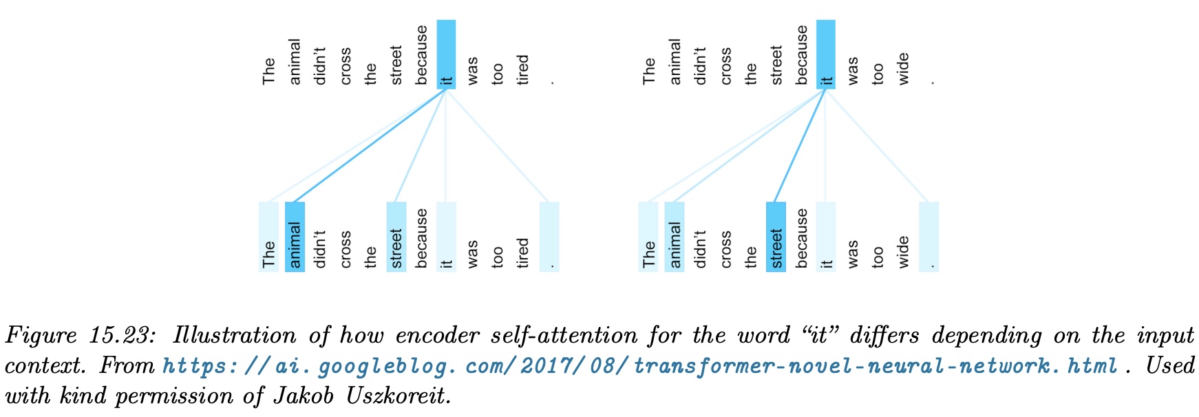
- Attention lets one point of the input be strongly influenced by others in a context-dependent way
- See the above, which associates the word “it” with “animal” when the pronoun needs to be interpreted in context
Token Prediction
- Recall with the ChatGPT style prediction of the next token, we need to find a \({\mathbb{P}\left( {x_t}\left| {x_{t-1}, x_{t-2}, \ldots, x_1} \right. \right)}\)
- Where \(t\) might be \(1{-}2\) million or more, and there might be \(100{,}000\) possible discrete \(x_t\) values
- Attention is central because it can find representations of the \(x_{t-1}, x_{t-2}, \ldots, x_1\) for conditioning
- Self-attention makes it possible for the representations to capture the features of the joint distribution of previous tokens
Example: Attention for Cross-Sectional Data
Attention as Learned Peer Comparison
- Task: predict each firm \(i\)’s next-quarter return \(y_i\) using the cross-section of \(n\) firms with features \(x_i \in {\mathbb{R}}^h\) (size, leverage, sector, R&D, ROA)
- Without attention: pick peers by SIC code, average their returns — a weighted average \(\hat{y}(x) = \sum_i \alpha_i y_i\) where \(\alpha_i \propto K(x, x_i)\) and \(K\) is a fixed smoothing kernel
- With attention: learn the similarity function, and what firm \(i\) considers “similar” can differ from what firm \(j\) considers “similar”
What the Projections Capture
- Task reminder: predict firm \(i\)’s return using information gathered from other firms
- \(W_K x_j\) = firm \(j\)’s profile: how it presents itself to others (sector, size, growth characteristics)
- \(W_Q x_i\) = firm \(i\)’s search criterion: what features firm \(i\) looks for in peers to help predict its own return
- \(q_i \cdot k_j\) = how well firm \(j\)’s profile matches firm \(i\)’s search criterion → attention weight \(\alpha_{ij}\)
- \(W_V x_j\) = the information firm \(j\) contributes (its return, transformed) — weighted by \(\alpha_{ij}\) and summed
- Asymmetry from \(W_Q \neq W_K\): a startup searching for peers loads on “large, established, tech” → high \(\alpha_{\text{startup},\text{Apple}}\). But Apple searching for peers loads on “mega-cap, global” → low \(\alpha_{\text{Apple},\text{startup}}\). The attention weights are inherently directional
Attention vs Self-Attention for Firms
- Cross-attention: target portfolio firms query a separate reference universe to predict their returns. One-directional: targets search, references answer
- Self-attention: all \(n\) firms in one pool. Every firm simultaneously queries and is queried. Produces the full \(n \times n\) peer-relevance network
- Self-attention adds structure:
- Same \(W_Q, W_K\) must work for every firm as both searcher and reference → learns general relevance, not ad-hoc pairings
- Asymmetric: \(\alpha_{ij} \neq \alpha_{ji}\) — firm \(i\) finding firm \(j\) useful for prediction doesn’t imply the reverse
- Stacked layers: firm \(i\)’s representation is enriched by its peers, whose representations were enriched by their peers — captures indirect peer effects (\(i \leftarrow j \leftarrow k\))
- Progression: fixed kernel (manual SIC peers) → attention (learned one-directional lookup) → self-attention (learned, asymmetric, full peer network)
The Transformer Block
From Attention to Transformers
- Attention is a linear re-weighting of values — powerful for routing information, but limited on its own
- To build a full sequence model we need three additional ideas:
- Nonlinearity: a feed-forward network (FFN) after attention to transform representations
- Gradient flow: residual (skip) connections so gradients pass through 100+ layers
- Training stability: layer normalization to keep activations well-scaled
- Together with multi-head attention, these form the transformer block — the repeating unit of every modern LLM
Feed-Forward Network (FFN)
- Applied independently to each token after attention: \[
\text{FFN}(z) = W_2\,\sigma(W_1 z + b_1) + b_2
\]
- \(W_1 \in {\mathbb{R}}^{d_{\text{ff}} \times d}\) with \(d_{\text{ff}} \approx 4d\); \(\sigma\) = ReLU or GELU (recall Deep Learning lecture)
- Why is this needed? Attention output is linear in \(V\) — it routes information but doesn’t transform it
- Intuition:
- Attention = “communicate between tokens”
- FFN = “think about what you heard”
Residual Connections
- An econometrician’s instinct: instead of modeling the level \(z_{\text{out}} = f(z_{\text{in}})\) directly, model the residual \[
z_{\text{out}} = z_{\text{in}} + f(z_{\text{in}})
\]
- The network only needs to learn the correction \(f\) — the deviation from the identity
- Easy to learn “do nothing” (set \(f \approx 0\)), hard to learn the identity with a general \(f\)
- Gradient: \(\frac{\partial z_{\text{out}}}{\partial z_{\text{in}}} = I + \frac{\partial f}{\partial z_{\text{in}}}\)
- Even if \(\frac{\partial f}{\partial z_{\text{in}}} \approx 0\), gradients still flow through \(I\) — prevents vanishing gradients across 100+ layers
- This is the “Add” in the “Add & Norm” boxes in the architecture diagram
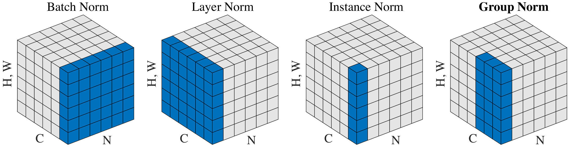
Why Layer Normalization?
\[ \text{LayerNorm}(z) = \gamma \odot \frac{z - \mu_z}{\sqrt{\sigma_z^2 + \epsilon}} + \beta \]
- An engineering necessity forced by finite-precision arithmetic
- Through many layers, activations drift to very large or very small values
- Gradients accumulate numerical errors → training becomes unstable
- Normalization recenters activations into a well-behaved range after every sub-layer
- Normalizes across features (per token), not across the batch
- Sequences have variable length → batch statistics are unreliable → LayerNorm over BatchNorm
- This is the “Norm” in “Add & Norm”; \(\gamma, \beta\) are learnable scale and shift
The Transformer Block
\[ \begin{aligned} z' &= \text{LayerNorm}\!\bigl(x + \text{MultiHead}(x)\bigr) \\ z_{\text{out}} &= \text{LayerNorm}\!\bigl(z' + \text{FFN}(z')\bigr) \end{aligned} \]
Data flow (one block):
Input → Multi-Head Attention → Add residual → LayerNorm → FFN → Add residual → LayerNorm → Output
- Stack \(L\) identical blocks (\(L = 12\) for BERT-base, \(L \geq 96\) for GPT-4 class)
- Each block has its own learned parameters
- Dropout (not shown) is applied after attention and FFN for regularization
![]()
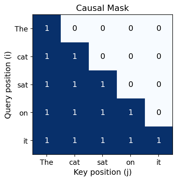
Why Causal Masking?
- Goal: learn representations from raw text with no labels (self-supervised)
- Key idea: use each sequence as its own training data — predict every next token from its history
- The causal mask enforces this: \[ \text{Attn}(Q, K, V) = \mathrm{softmax}\!\left(\frac{Q K^\top}{\sqrt{d}} + M\right) V \] where \(M_{ij} = 0\) if \(i \geq j\), and \(M_{ij} = -\infty\) if \(i < j\)
- After softmax, \(e^{-\infty} = 0\): token \(i\) attends only to tokens \(1, \ldots, i\)
- This is the “Mask (opt.)” in the architecture diagram
- Enables parallel training: all positions are predicted simultaneously, each seeing only its past
- Different masking strategies → different self-supervised objectives (e.g., BERT masks random tokens instead → bidirectional context)
Transformer Architectures
Example Encoder-Decoder Transformer Architecture
Sequence to Sequence
- Early transformer designed for translation tasks (sequence of tokens as input to sequence of tokens as output)
- i.e., the \({\mathbb{P}\left( {y_1, \ldots, y_T}\left| {x_1, \ldots, x_T} \right. \right)}\) where \(T\) might be enormous, and \(x,y\) might allow tens of thousands of tokens
- The design of these typically uses a transformer to encode \(x_1, \ldots, x_T\) into a representation, then another to decode, and take the representation back to the \(y_1, \ldots, y_T\) tokens
- Encoder: bidirectional self-attention (no mask) — every input token sees all others
- Decoder: causal self-attention + cross-attention where \(Q\) comes from decoder, \(K\) and \(V\) from the encoder output
- This cross-attention is the middle attention block in the decoder stack (see diagram)
Decoder-Only Transformer
- To generate text token by token, as in sequential generation, we can use a single transformer
- i.e., the \({\mathbb{P}\left( {x_{T+1}}\left| {x_1, \ldots, x_T} \right. \right)}\)
- This is GPT, LLaMA, Claude, Gemini, and most modern LLMs
- Training: predict every next token in parallel using causal masking (no future leakage)
- Trained with cross-entropy loss (MLE), exactly as in the Embeddings lecture
- Simpler than encoder-decoder: no cross-attention needed, just stacked masked self-attention blocks
- Scales well — architecture and data can grow together
Encoder-Only Transformer
- For tasks like classification, the transformer can be used to encode an internal representation of the input for a downstream task
- i.e., the \({\mathbb{P}\left( {\text{Class}(x_1, \ldots, x_T) = C_i}\left| {x_1, \ldots, x_T} \right. \right)}\)
- Bidirectional self-attention (no causal mask) — every token sees the full context
- Self-supervised via Masked Language Modeling (MLM): mask ~15% of tokens, predict them from context
- This is the
[MASK]fill-in task and the word embeddings from the Embeddings lecture
- This is the
- BERT is the canonical example — now clear why it uses bidirectional attention: it needs context on both sides of each masked token
- The final layer representation feeds into a classifier head for the downstream task
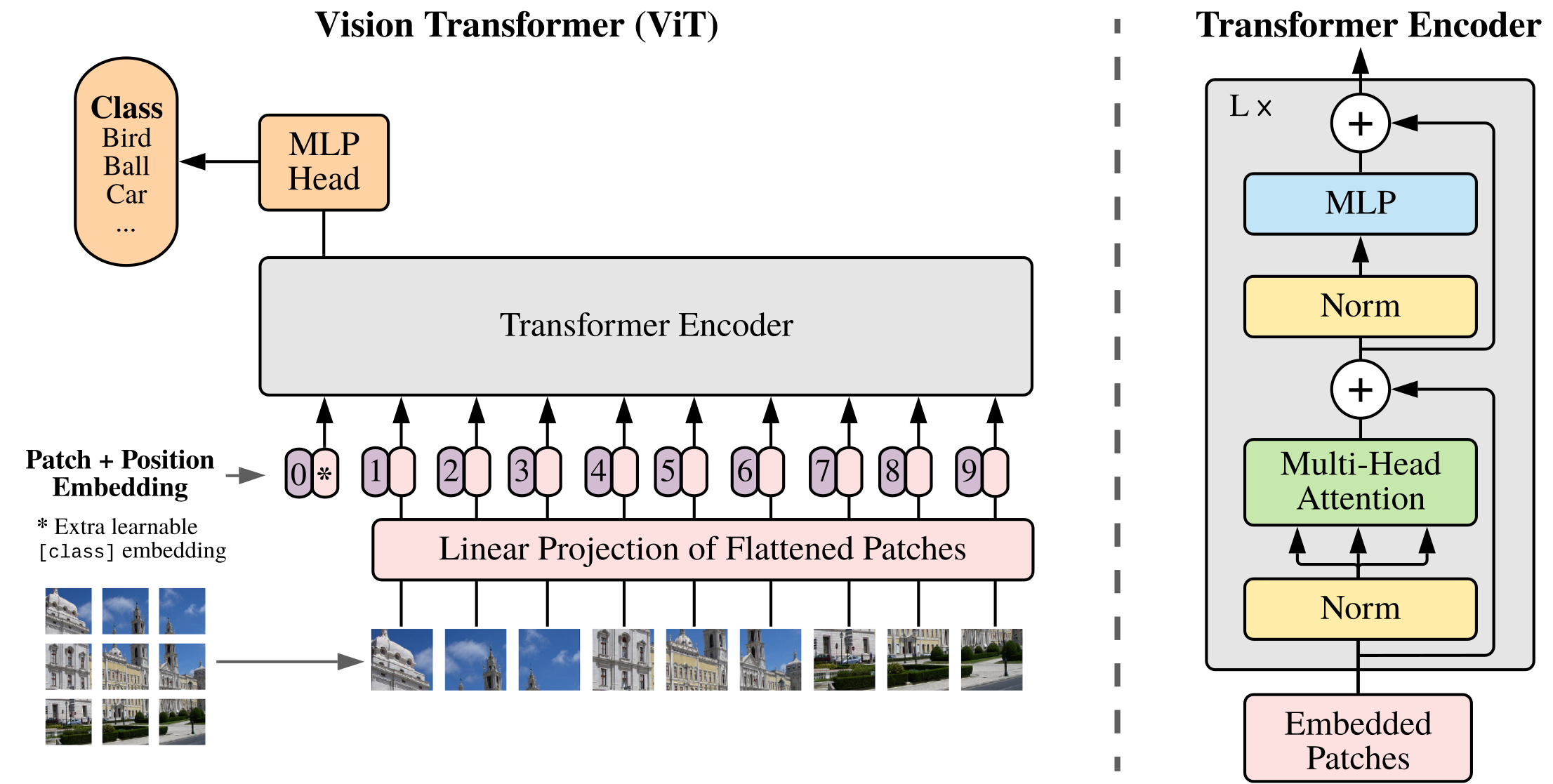
Vision Transformers (ViT)
- Split the image into fixed-size patches (e.g., 16×16 pixels)
- Flatten each patch and linearly project to embedding dimension \(d\)
- Add learned 2D positional embeddings
- Prepend a
[CLS]token whose final representation is used for classification
- Key insight: a transformer is a general-purpose sequence processor, not NLP-specific
Beyond Images and Text
- The attention mechanism applies whenever parts of the data should inform each other
- Examples beyond NLP and vision:
- Graphs: Graph Attention Networks (GATs) use attention over node neighbors
- Time series: temporal attention for forecasting and anomaly detection
- Proteins: AlphaFold uses attention over amino acid residues to predict 3D structure
- General pattern: tokenize your domain → add appropriate positional info → apply transformer blocks