import os
os.environ["TOKENIZERS_PARALLELISM"] = "false"  # Avoid warning with Quarto
os.environ["HF_HUB_DOWNLOAD_TIMEOUT"] = "120"  # Increase timeout for CI
import openai
import transformers
import torch
from torch.nn.functional import cosine_similarity
from openai import OpenAI
from transformers import pipeline, AutoTokenizer, AutoModel # Hugging Face
from sklearn.manifold import TSNE
import matplotlib.pyplot as plt
import numpy as npEmbeddings, NLP, and LLMs
Machine Learning Fundamentals for Economists
Overview
Summary
- Relate embeddings to autoencoders and representation learning
- Discuss text and other embeddings
- Better discuss “out of distribution”, transfer learning, and fine tuning
- Introduce self-supervised learning and semi-supervised learning
- Use the OpenAI and Hugging Face Packages
- Prepare to discuss attention and the transformer architecture and foundation models in the next lecture
References
- These notes are a bare-bones introduction. See references for more
- See Melissa Dell’s Survey Deep Learning for Economists and Course
- ProbML Book 1 and ProbML Book 2
Packages
Introducing new packages from OpenAI and Hugging Face
OpenAI
- Sign up for the OpenAI Platform
- Free for limited numbers of “tokens”
- Go to the
API keystab and create a key - In your terminal, set
OPENAI_API_KEYto this value (see here)
Is (Some) ML Just Fancy Logit?
Discrete Random Variables
- Up until now, we have mostly been interested in continuous outputs from our models
- When working with NLP/etc. we usually have discrete outputs such as a classification or prediction of the next “token”
- Let’s review basic econometrics of logit and classification problems and explain how they work with learned representations
Logit and Classification
- Logit takes observables \(X\), a binary outcome \(Y\) from some population distribution and coefficients \(\beta\) \[
{\mathbb{P}\left( {Y = 1}\left| {X} \right. \right)} = \frac{\exp(X\cdot \beta)}{1 + \exp(X\cdot \beta)}
\]
- In the background is a population distribution \(\mu^*\) over \((Y,X)\)
- The parameters \(\beta\) are usually estimated with maximum likelihood with samples from \(\mu^*\) (e.g., equivalent to ERM for regression)
- \(X\) are handpicked observables, often transformed by economists (e.g., “feature engineering” in ML-jargon)
Multinomial Logit
- More generally, with \(C\) possible outcomes, we have a multinomial logit model \[ {\mathbb{P}\left( {Y = c}\left| {X} \right. \right)} = \frac{\exp(X\cdot \beta_c)}{\sum_{c'=1}^C \exp(X\cdot \beta_{c'})} \]
- The \(\beta\) (matrix) are usually estimated with maximum (log)-likelihood \[ \min_{\beta}\left\{- \sum_{(X, y)\in{\mathcal{D}}} \log {\mathbb{P}\left( {Y = y}\left| {X;\beta} \right. \right)}\right\} \]
Nesting Representations
- Often best to think of deep-learning as finding good representations of the data, \(\phi : {\mathcal{X}}\to {\mathcal{Z}}\) and then a thin mapping or projection of that representation to an outcome space, \(\hat{f} : {\mathcal{Z}}\to {\mathcal{Y}}\)
- With discrete-valued multinomial logit maps to a distribution over \(C\) outcomes, \({\mathcal{Y}}= \{1, \ldots, C\}\) \[
{\mathbb{P}\left( {Y = c}\left| {X;\beta,\theta} \right. \right)} = \frac{\exp(\phi(X;\theta)\cdot \beta_c)}{\sum_{c'=1}^C \exp(\phi(X;\theta)\cdot \beta_{c'})}
\]
- Then MLE: \(\min_{\beta, \theta} \left\{- \sum_{(X, y)\in{\mathcal{D}}} \log {\mathbb{P}\left( {Y = y}\left| {X;\beta, \theta} \right. \right)}\right\}\)
- As always, with ML we can just nest the \(\phi\) and \(\hat{f}\) in the same function to jointly optimize all parameters
Turning “Features” to Probabilities
- Common to have a complicated internal approximation which they want to convert to a discrete action/state/prediction/classification
- The easiest approach, pervasive in ML methods, is to convert this to a probability distribution over discrete outcomes
- “softmax”, i.e. the multinomial logit PMF, provides an easy way to do this
- Among other reasons, this makes the objective function differentiable and allows for gradient-based optimization
Is ML Just Fancy Logit?
- At this point many economists will say that this all just sounds like fancy logit
- That is mostly true, for this type of problem
- But that is not an insult! Multinomial logit is powerful, and MLE is well understood. Logit/LLS/etc. are simple ML methods
- The key difference with deep learning + logit is important:
- Economists typically work with engineered representations (e.g., taking logs, first-differences, variable selection)
- But deep learning lets us use learned representations, \(\phi(X;\theta)\)
Classic ML Approaches with LASSO
- Worth contrasting to a “classic” ML. If the “features/observables” of \(X\) are:
- Assumed to map to the output probabilities linearly
- Likely to overfit, or not be identified, by using irrelevant features
- Then you can do things like a LASSO regularized multinomial logit \[
\min_{\beta} \left\{- \sum_{(X, y)\in{\mathcal{D}}} \log {\mathbb{P}\left( {Y = y}\left| {X;\beta} \right. \right)} + \lambda ||\beta||_1\right\}
\]
- i.e., penalize the 1-norm of the coefficients, which encourages sparsity of \(\beta\) for \(\lambda > 0\). Deep Learning often achieves this regularization indirectly (as discussed in the Overparametrization lecture)
Terminology Differences
- Standard MLE loss in this setup is the “cross-entropy loss”
- The formula for the multinomial logit is called the “softmax” function
- When thinking about the separate mapping of the representation to the output, we often think of it as the last layer
- And remember that we can have representations in the latent space:
- If there are \(N\) observables to predict \(C\) outcomes, then in multinomial logit we estimate \(N \times C\) parameters
- But with representations, \(z = \phi(X;\theta)\), it might be a much higher (or lower) dimensional mapping to \(C\) outcomes
- Confusion: “Inference” in some ML-speak is simply evaluating \(f(X)\)
Embeddings
What is an Embedding?
What is an Embedding?
- An embedding is a numerical representation of an object (such as a word, phrase, or image) in a continuous vector space, allowing for the capture of semantic relationships and similarities between the objects.
- In natural language processing, word embeddings like Word2Vec or GloVe translate words into high-dimensional vectors, making it easier for algorithms to process and understand linguistic context.
Latent Space
completion = client.chat.completions.create(model="gpt-4o-mini",
    messages=[
        {
          "role": "system",
          "content": "You provide 2 short bullet points, technical answers."
        },
        {
          "role": "user",
          "content": "What is an embedding?"
        },
        {
          "role": "assistant",
          "content": "- An embedding is a dense vector representation of objects, such as words, sentences, or images, that captures semantic meanings and relationships in a continuous vector space.\n- It transforms high-dimensional data into a lower-dimensional format while preserving essential properties, enabling easier computation in machine learning tasks."
        },
        {
          "role": "user","content": "What is the relationship to latent spaces?"
        },
    ]
)
print(completion.choices[0].message.content)
Latent Space
- Embeddings are often used to map data points into latent spaces, where each point's position reflects its intrinsic properties and relationships within the dataset.
- Latent spaces represent compressed and abstract features of the data, enabling efficient clustering, visualization, and downstream tasks like classification or generation.
Detour into OpenAI (others are similar)
- This is making calls to the OpenAI API.
- Three roles:
- system: setup for the LLM to establish the persona, how to respond, etc.
- user: the question or prompt
- assistant: the response
- Note that in a sequence of calls, we give the entire history including its own responses (tagged as
assistant) - We will come back to this shortly. Think of this as information for conditioning.
Embeddings Overview
- Used loosely and inconsistently, but the spirit is the same
- A mapping of some \(x \in {\mathcal{X}}\) to a latent space \(\phi(x) \in {\mathcal{Z}}\)
- Typically we want that \({\mathcal{Z}}\) as a continuous vector space of finite dimension
- Crucially, we can think of distances in that space (e.g., \(||\phi(x) - \phi(y)||\))
- The dimension of \({\mathcal{Z}}\) may be smaller or larger than \({\mathcal{X}}\)
- If larger, typically embeddings of data \(x \in \mu^*\) are close to a lower-dimensional manifold in \({\mathbb{R}}^3\) (e.g., recall the kernel trick)
- Sometimes, as with network embeddings, want to preserve norms
- e.g. if \(||x - y||\) is small, then \(||\phi(x) - \phi(y)||\) is small
Inner Products Implicitly Define Norms (and Embeddings)
- As we saw with kernels, the embedding may be implicit in an inner product
- Kernels induce norms without explicitly forming the feature map, \(\phi(x)\), to the embedding space—which would be defined implicitly by \(K(x, x') = \phi(x)^T \phi(x')\).
- As discussed, the benefit of kernel methods is that the embedding space may be infinite dimensional, but the kernel is finite dimensional. The cost is we cannot directly map \(x\) to the embedding space
Cosine Similarity
- Canonical case of an inner product (with an associated norm, etc.)
- Cosine similarity is the “angle” between two vectors in the embedding space \(z = \phi(x)\) and \(z' = \phi(x')\) \[ \mathrm{sim}(z, z') = \frac{z \cdot z'}{||z|| ||z'||} \]
- Interpretation: If \(z\) and \(z'\) are
- close in the embedding space, then the cosine similarity is close to 1
- orthogonal, then the cosine similarity is 0
- opposite, then the cosine similarity is -1
- Norm comparison \(||z - z'||\) instead? Works but not invariant to scaling
Learned vs. Engineered Embeddings
- Embeddings are not related to a specific “supervised” goal, and there may be many useful embeddings for a given data set
- We could engineer them (explicitly or implicitly).
- e.g., count frequency of words in text, define implicitly through a kernel
- Or we can learn them
- e.g., representation learning in a NN, PCA, etc.
- Recall that when we fit a neural network, \(f(x) = \hat{f}(\phi(x))\), we can think of \(\phi(x)\) as an embedding of \(x\) in a latent space mapped to output by a shallow \(\hat{f}\)
Autoencoders and Compression
- One sense of “optimality” of embeddings is whether you can find a representation which best compresses the data in a finite dimensional latent space (or a higher-dimensional latent space with a low-rank structure)
- This underlies the idea of using an Autoencoder. See ProbML Book 1 Section 20.3 and ProbML Book 2 Section 21
- The idea is to find functions which “encode” the data into a latent space, and then “decode” it back to the original space
Autoencoders and Dimensionality Reduction
- General class of problems which they call auto-encoders in ML/data science
- Function \(f\), the encoder, maps \(X\) to a latent space \(Z\), which may be lower-dimensional
- Function \(g\), the decoder, maps points in the latent space \(Z\) back to \(X\)
- \(\theta_e\) and \(\theta_d\) are parameters for \(f\) and \(g\) which we are trying to find
- Then the goal is to find the \(\theta_e\) and \(\theta_d\) parameters for our encoder, \(f\), and decoder, \(g\), where for as many \(X\) as possible we have
\[ g(f(x; \theta_e); \theta_d) \approx x \]
- The \(z = f(x;\theta_e)\) may or may not be lower-dimensional
Optimization Problem for an Autoencoder
If we had a distribution for \(x\) then can solve
\[ \min_{\theta_e, \theta_d} {\mathbb{E}_{{x\sim \mu^*}}\left[ {||g(f(x; \theta_e); \theta_d) - x||_2^2} \right]} \]
Fit with ERM for \({\mathcal{D}}\sim \mu^*\)
\[ \min_{\theta_e, \theta_d} \frac{1}{|{\mathcal{D}}|} \sum_{x \in {\mathcal{D}}} ||g(f(x; \theta_e); \theta_d) - x||_2^2 \]
PCA as the Optimal Linear Autoencoder
- Let \(f(x) = W^T x\) and \(g(z) = W z\) where \(W \in {\mathbb{R}}^{M \times L}\). If \(\hat{x} \approx W W^T x\), “reconstruction error” is \(||\hat{x} - x||_2^2\).
\[ \min_{W} \frac{1}{N} \sum_{n=1}^N ||W \overbrace{W^T x_n}^{z_n = f(x_n;W)} - x_n||_2^2,\quad \text{with } W^T W = I \]
Word Embeddings
Tokens and Vocabulary
- Rather than trying to embed individual characters, it is usually better to encode entire words (and, later, sentences, paragraphs, text+images, etc.)
- If we decide on something that separates them, e.g. whitespace, then we can map words to an integer index for each word
- Let’s use a prebuilt tokenizer from Hugging Face. With a different type of data (e.g., historical data) you may want to customize what a “word” is
Tokens and Vocabulary
['hello', ',', 'hugging', 'face']
[7592, 1010, 17662, 2227]
Token IDs to Embeddings
- The discrete values for the different words are not inherently comparable
- An embedding will put them in a space where we can consider similarity
- For now, let’s use an embedding from a prebuilt “model”
model = AutoModel.from_pretrained("bert-base-uncased")
def get_embedding(sentence):
    tokens = tokenizer(sentence, return_tensors="pt")
    with torch.no_grad():
        outputs = model(**tokens)
        embeddings = outputs.last_hidden_state
        # will see there are 3 total tokens, only middle is the sentence
        return outputs.last_hidden_state[0,1:-1,:].squeeze()
embed = get_embedding("hello")
print(embed.shape)torch.Size([768])Similarity
- Measure distances in embedding space with cosine similarity or norms
- Because we are in higher-dimensions, there can be different reasons for similarity. e.g., bank for money vs. the bank of a river, but river and money are not as similar
embed_bank = get_embedding("bank")
embed_banks = get_embedding("banks")
embed_river = get_embedding("river")
embed_money = get_embedding("money")

print(f"sim(bank, banks) = {cosine_similarity(embed_bank, embed_banks, dim=0)}")
print(f"sim(bank, river) = {cosine_similarity(embed_bank, embed_river, dim=0)}")
print(f"sim(bank, money) = {cosine_similarity(embed_bank, embed_money, dim=0)}")
print(f"sim(river, money) = {cosine_similarity(embed_river, embed_money, dim=0)}")
sim(bank, banks) = 0.7438120245933533
sim(bank, river) = 0.5635620951652527
sim(bank, money) = 0.6932224035263062
sim(river, money) = 0.5209330916404724Where Did the Embedding Come From?
- As we will see below,
bert-base-uncasedis a model which can predict missing words as its “supervised” goal, \(f(x) = \hat{f}(\phi(x))\) - This code just ripped off the \(\hat{f}(\cdot)\) layers and use the latent space \(\phi(x)\)
- It is important to get a sense of how the representations were learned - as they may not be appropriate for your task
Using OpenAI API
def get_openai_embedding(sentence):
  response = client.embeddings.create(input = [sentence], model="text-embedding-3-large")
  return torch.tensor(response.data[0].embedding)

embed_bank = get_openai_embedding("bank")
embed_banks = get_openai_embedding("banks")
embed_river = get_openai_embedding("river")
embed_money = get_openai_embedding("money")
print(f"sim(bank, banks) = {cosine_similarity(embed_bank, embed_banks, dim=0)}")
print(f"sim(bank, river) = {cosine_similarity(embed_bank, embed_river, dim=0)}")
print(f"sim(bank, money) = {cosine_similarity(embed_bank, embed_money, dim=0)}")
print(f"sim(river, money) = {cosine_similarity(embed_river, embed_money, dim=0)}")
sim(bank, banks) = 0.7882463335990906
sim(bank, river) = 0.41433995962142944
sim(bank, money) = 0.4347141981124878
sim(river, money) = 0.37470367550849915Bigger Embeddings
Bag of Words
- Words usually occur in sentences, paragraphs, etc.
- Instead of embedding a single word, we can embed a block of text.
- Simple starting point: compare the relative frequency of words
- Turn the text into blocks of tokens with unique identifiers
- Filter out tokens that are not useful (e.g., “the”, “a”, etc.)
- Count the frequency of each token
- The embedding is the vector of the frequency of each token
- Many issues with this, but crucially it does not capture any sense of context dependent meaning of words, and is invariant to word order
Sentence Embeddings with LLMs
- Encode an entire sentence (i.e., a sequence of tokens) into a single embedding and compare for similarity
- Since individual words are embedded, we just average for the sentence
e_1 = get_embedding("The man bites the dog").mean(dim=0)
e_2 = get_embedding("The dog chased the man").mean(dim=0)
e_3 = get_embedding("The man was chased by the dog").mean(dim=0)
print(f"sim(e_1, e_2) = {cosine_similarity(e_1, e_2, dim=0)}")
print(f"sim(e_1, e_3) = {cosine_similarity(e_1, e_3, dim=0)}")
print(f"sim(e_2, e_3) = {cosine_similarity(e_2, e_3, dim=0)}")
sim(e_1, e_2) = 0.8429716229438782
sim(e_1, e_3) = 0.8270692229270935
sim(e_2, e_3) = 0.9152544736862183- Note that the 2nd and 3rd are the most similar, and the 1st and 3rd the least.
What About the OpenAI API?
e_1 = get_openai_embedding("The man bites the dog")
e_2 = get_openai_embedding("The dog chased the man")
e_3 = get_openai_embedding("The man was chased by the dog")
print(f"sim(e_1, e_2) = {cosine_similarity(e_1, e_2, dim=0)}")
print(f"sim(e_1, e_3) = {cosine_similarity(e_1, e_3, dim=0)}")
print(f"sim(e_2, e_3) = {cosine_similarity(e_2, e_3, dim=0)}")
sim(e_1, e_2) = 0.5413669943809509
sim(e_1, e_3) = 0.5226994156837463
sim(e_2, e_3) = 0.7910534143447876- Same ordering. A good sign.
Be Cautious, Interpretation is Tricky
e_1 = get_openai_embedding("The man bites the dog")
e_2 = get_openai_embedding("The dog chased the man")
e_3 = get_openai_embedding("The man was chased by the dog")
e_4 = get_openai_embedding("The man chased the dog")
print(f"sim(e_1, e_2) = {cosine_similarity(e_1, e_2, dim=0)}")
print(f"sim(e_1, e_3) = {cosine_similarity(e_1, e_3, dim=0)}")
print(f"sim(e_2, e_3) = {cosine_similarity(e_2, e_3, dim=0)}")
print(f"sim(e_3, e_4) = {cosine_similarity(e_3, e_4, dim=0)}")
sim(e_1, e_2) = 0.5413559079170227
sim(e_1, e_3) = 0.5226873159408569
sim(e_2, e_3) = 0.7911072373390198
sim(e_3, e_4) = 0.8597927093505859- Note that
sim(e_3, e_4) > sim(e_3, e_2)even though they seem to have the exact opposite meaning! - Why? There are many embeddings (e.g. bag of words) which make these close, and others where they are far apart. Hard to know without a sense of how it was trained.
Clustering
- Since embeddings provide a measure of similarity/distance, we can cluster it into groups or use other tools to find interpretations
- There are various algorithms to cluster based on representations, and find the closest elements within the set of data for a new element
- One approach: come up with a lower-dimensional embedding which preserves norms, as in t-SNE (t-Distributed Stochastic Neighbor Embedding)
- i.e., find a \(h(\cdot)\) such that if \(||x - y||\) is small, then \(||h(x) - h(y)||\) is small
- Generally better than k-means, etc. for this kind of problem, and allows you to project to 2 or 3 dimensional embeddings, not just discrete values
Get Some Random Embeddings
vocab = tokenizer.get_vocab()
tokens = list(vocab.keys())
print(f"model has {len(tokens)} tokens")
special_tokens = ['##', '[MASK]', '[CLS]', '[SEP]', '[PAD]']
full_tokens = [token for token in tokens if not token.startswith('##') and token not in special_tokens]
print(f"model has {len(full_tokens)} full tokens (e.g. not special symbols, special tokens, etc.)")
sampled_tokens = np.random.choice(full_tokens, size=50, replace=False)
token_ids = [vocab[token] for token in sampled_tokens]
with torch.no_grad():
    embeddings = model.embeddings.word_embeddings(torch.tensor(token_ids))
model has 30522 tokens
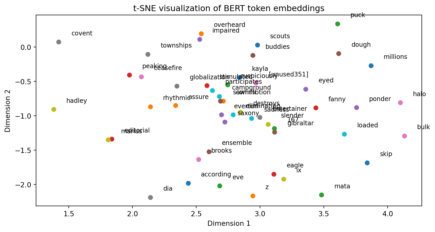
model has 24690 full tokens (e.g. not special symbols, special tokens, etc.)Visualize with t-SNE
tsne = TSNE(n_components=2, random_state=0) # approx with 2 dim embedding
embeddings_2d = tsne.fit_transform(embeddings.numpy())
# Plot the t-SNE results
plt.figure()
for i, token in enumerate(sampled_tokens):
    x, y = embeddings_2d[i]
    plt.scatter(x, y)
    plt.text(x+0.1, y+0.1, token, fontsize=9)
plt.title('t-SNE visualization of BERT token embeddings')
plt.xlabel('Dimension 1')
plt.ylabel('Dimension 2')
plt.show()
Visualize with t-SNE
Lowering the Embedding Dimension
- As discussed, t-SNE is one way to project down to something visualizable
- More generally, though, you can find a lower-rank approximation to the embedding space
- With some APIs, (e.g. OpenAI) they make this especially easy
- In particular, you can simply drop digits of precision on the embedding to make it coarser, following this paper
- See OpenAI docs for more details. Can do this automatically by passing
dimensions
Classification
- For classification tasks, we can use this embedding with representation learning and softmax (i.e., logit likelihood)
- One strategy for classification
- Embed sentences
- Use some nonlinear transformations (e.g., NN) to get a representation of the embedding
- Use a “softmax” to get a probability distribution over the classes
- Fit with MLE as a “supervised” (multinomial logit) problem
- Others use embeddings as inputs to different classification algorithms (e.g. OpenAI random forest example)
Multi-Modal Embeddings
- Embeddings can be used for more than just text
- Images, audio, etc. can all be embedded
- The key is to have a representation which is useful for the task at hand
- For example, we can embed text and images together to predict the sentiment of a review
Aligning Embeddings
- Loosely, if you have related data on the same entities (e.g., labels on images) then you can work to align the embeddings of both
- e.g., a \(\phi_1(X_{\text{image}})\) and \(\phi_2(X_{\text{text}})\) similar if the text describes the image
- Then you can attempt to get the \(\phi_1\) and \(\phi_2\) to be similar for that data
- If so, then you can map back and forth between image and text in the embedding space (i.e., take text, map to \(\phi_2\) to the embedding space, then map back from the embedding to the image space)
- See Melissa Dell’s Multimodal Learning. Complicated in practice (e.g., contrastive learning)
- See OpenAI’s multimodal example with CLIP for an example
Sequential Data and Token Prediction
Distribution of “Tokens”
- In many cases, data has an inherent sequential ordering. e.g. time series, language, etc.
- Consider conditional probabilities over \(x_t \in {\mathcal{X}}\) which is discrete set of outcomes \(c = 1, \ldots C\). Generically call these “tokens”
- Objects of interest: for \(x_1, x_2, \ldots, x_T\) for a sequence of length \(T\), have a “population distribution”, \((x_1, \ldots, x_T) \sim \mu^*\)
- We may want to condition on the past to predict the next token, condition on the entire sequence to predict missing ones, etc.
Token Prediction from Conditional Probabilities
- Given a sequence \(x_1, x_2, \ldots, x_{t-1}\), model the conditional distribution: \[
{\mathbb{P}\left( {x_t}\left| {x_{t-1}, x_{t-2}, \ldots, x_1} \right. \right)}
\]
- Where in the background these are done with marginal and conditional probabilities sampling the population distribution \(\mu^*\)
- Basic strategy (details on “transformers” after we see how to use them):
- Do an embedding for each token \(\phi_1(x_t)\)
- Map those embeddings to some combined representation, \(\phi_2(\phi_1(x_1), \ldots, \phi_1(x_{t-1}))\)
- Map that with “softmax” to get probabilities over \(c = 1, \ldots, C\) for \(x_t\)
- Fit with MLE as a “supervised” (multinomial logit) problem
Provide Conditioning Tokens in the Prompt
- See Melissa Dell’s Prompting lecture, Hugging Face’s docs and Prompts for Economists
client = OpenAI()
completion = client.chat.completions.create(
    model="gpt-4o-mini",
    temperature=0.7, # higher temperature adds "entropy"
    messages=[
        {
          "role": "system",
          "content": "You provide 2 short bullet points, technical answers."
        },
        {
          "role": "user",
          "content": "What is an embedding?"
        }
    ]
)
print(completion.choices[0].message.content)
Provide Conditioning Tokens in the Prompt
- An embedding is a mathematical representation of discrete objects, such as words or images, in a continuous vector space, enabling them to capture semantic relationships and similarities.
- In machine learning, embeddings are often used to transform categorical data into dense vectors that can be processed by algorithms, improving performance in tasks like natural language processing and recommendation systems.
Concatenating Results
completion = client.chat.completions.create(model="gpt-4o-mini",
    messages=[
        {
          "role": "system",
          "content": "You provide 2 short bullet points, technical answers."
        },
        {
          "role": "user",
          "content": "What is an embedding?"
        },
        {
          "role": "assistant",
          "content": "- An embedding is a dense vector representation of objects, such as words, sentences, or images, that captures semantic meanings and relationships in a continuous vector space.\n- It transforms high-dimensional data into a lower-dimensional format while preserving essential properties, enabling easier computation in machine learning tasks."
        },
        {
          "role": "user","content": "What is the relationship to latent spaces?"
        },
    ]
)
print(completion.choices[0].message.content)
Concatenating Results
- Embeddings reside in latent spaces, which are lower-dimensional representations of input data, allowing for the capture of hidden patterns and structures.
- Latent spaces are a more general concept that encompasses various types of dimensional reductions, while embeddings specifically refer to learned representations for particular data types in machine learning.
Mental Model of Sequential Generation
- Start with a set of tokens, \(x_1, x_2, \ldots, x_{t-1}\) (include EVERYTHING)
- Condition on those tokens to find the \({\mathbb{P}\left( {x_t}\left| {x_{t-1}, x_{t-2}, \ldots, x_1} \right. \right)}\) distribution
- Sample from that to get the \(x_t\) token
- “Temperature” settings increases/decreases the entropy of \({\mathbb{P}\left( {x_t}\left| {\cdot} \right. \right)}\) artificially to encourage/discourage randomness
- Add its own generated token to the set of tokens, \(x_1, x_2, \ldots, x_{t-1}, x_t\)
- Condition on those tokens to find the \({\mathbb{P}\left( {x_{t+1}}\left| {x_t, x_{t-1}, \ldots, x_1} \right. \right)}\) distribution
- Repeat until it hits a special “done” token (itself predicted) or reaches a maximum length
Cardinality of the Estimated Conditional Distribution
- ChatGPT and others generate text token-by-token auto-regressively
- No Markov assumptions. \(C^T\) possible sequences of \(C\) tokens of length \(T\)
- Frontier LLMs circa 2025: \(C \approx 100{,}000\) tokens, context windows of \(T \approx 1{-}2\) million
- Estimating a \(\mathbb{P} : \{1, \ldots, C\}^{T+1} \to [0,1]\), where \(C^{T+1} \approx (10^5)^{10^6} = 10^{5 \times 10^6}\)
How Can This Possibly Work?
- It sometimes feels like it has compressed and memorized the entire internet
- We don’t always know the parameterization or number of tokens in the training data (remember, this largely uses MLE to train) but GPT-4 class models have
- \(|\Theta| \approx 1{-}2\) trillion parameters approximating \({\mathbb{P}\left( {\cdot}\left| {\cdot} \right. \right)}\)
- Trained on \(\approx 10{-}15\) trillion tokens of text data
- Which is a tiny amount of data given the cardinality of \(\mathbb{P}\)
- Paraphrasing Mikhail Belkin: like reconstructing an entire library from a molecule of ink.
- If the curse-of-dimensionality was the constraint, data would need to grow exponentially as \(T\) increases. It doesn’t.
Training
Manifold Hypothesis + Engineering Heroics?
- Plenty of interpretations for how this is possible, but a few key ones:
- The Manifold Hypothesis, as we discussed in the Deep Learning lecture.
- Given the right “representation”, human knowledge is far simpler than it appears. Knowledge is easily compressible since it has an inherent order independent of language
- Implicit and explicit regularization of various forms avoids overfitting
- The “Transformer”, a masterpiece of modern engineering we will discuss in our next lecture
- The Manifold Hypothesis, as we discussed in the Deep Learning lecture.
More than MLE
- While the lion’s share of this training may have been just sequentially predicting the next token for the data distribution, more is done in practice.
- e.g., “AI Alignment” which tries to encourage these models to capture socially desirable properties
- Encourage \(\mathbb{P}\) to be less racist or safer than the underlying training data by penalizing certain outcomes
- Add rewards based on human labeled data
- Distorting the \(\mu^*\) that you don’t want it to train with to ensure safety
- Reinforcement Learning from Human Feedback (RLHF). e.g. data from flagging an answer (good vs. bad) to help encourage good solutions
- And much more. An enormous undertaking for a big LLM.
Good Representations Are Reusable!
- As always, good representations tend to be useful for many tasks
- This goes both ways. Can use
- Different tasks can be used to refine the representations used for sequential prediction, even if not our primary goal
- Representations trained for LLMs for tasks which have nothing to do with their original training
- Crudely, can train a \(f(x) = \hat{f}(\phi(x))\) and swap out the \(\hat{f}\), or distort the \(\hat{f}\) to provide artificial incentives to encourage good \(\phi(\cdot)\)
- Whenever possible, start fitting a deep learning approximation from a previously trained one
Using “Unlabelled” Data
- In many cases, we have a lot of data, but only a small amount of labeled data (i.e., with outcomes)
- For example, there are many images, but we only have a few with human-coded descriptions
- Or we have a large number of examples of text for monetary policy statements, but only a few with human-coded sentiment or outcomes
- Given that most of the work in deep learning is finding the \(\phi(\cdot)\), how can we use the data itself to improve the representations - which will hopefully improve the model for many downstream tasks?
Semi-Supervised Learning
- Semi-supervised learning combines a small amount of labeled data with a larger set of unlabeled data to improve model performance by leveraging the structure in the unlabeled data.
- e.g., “Augment” data by adding noise, rotating images, for the labeled data we do have. This will add regularization, encourage important sources of representations (e.g., invariance to permutations)
Self-Supervised learning
- Self-supervised learning is a form of unsupervised learning where the model generates pseudo-labels or tasks from unlabeled data itself to learn useful representations without relying on external labels.
- e.g., mask out some words and predict them, mask out time-series data to predict the missing values, etc.
- See more in general surveys and ones on contrastive vs. generative
Contrastive Learning
- Contrastive learning is a form of self-supervised learning where the model is encouraged to keep the representations of similar data close, and dissimilar data further away.
- For example, with a batch of sentences, predict the next token for the sentence, but also try to predict the next token of the OTHER sentences in the loss (which should be unrelated/contrastive)
- This encourages the model to learn the importance of context. See SimCSE
Classification and Masking
Hugging Face
- Hugging Face provides a simple interface to many prebuilt transformer models, datasets, etc.
- We can use these for predicting the next token, but also tasks like sentiment analysis, filling in missing tokens, etc.
- Unlike the OpenAI API, we can download the models and use them locally, “fine-tune” them, etc.
- See Quick Tour for more
Pipelines
- The
pipelinefunction in Hugging Face is a simple way to use prebuilt models for common tasks. See the pipeline tutorial - Loads pretrained models from public repositories
Sentiment Analysis (defaults to “Positive” or “Negative”)
- Defaulted to
distilbert/distilbert-base-uncased-finetuned-sst-2-english
[{'label': 'POSITIVE', 'score': 0.9998424053192139}]
[{'label': 'NEGATIVE', 'score': 0.9997472167015076}]
[{'label': 'POSITIVE', 'score': 0.9997096657752991}]
[{'label': 'POSITIVE', 'score': 0.9587399959564209}]
[{'label': 'NEGATIVE', 'score': 0.8454722166061401}]- Not bad. But why is that
toy from the 80soverwhelmingly positive, andchicken crossed the roadmoderately negative?
Fill Masked
- Finds \({\mathbb{P}\left( {x_t}\left| {x_T, x_{T-1}, \ldots, x_{t+1}, x_{t-1}, x_{t-2}, \ldots, x_1} \right. \right)}\)
- Some, like BERT, were trained for this direct task
- Often done with a special
[MASK]token
[{'score': 0.04227164387702942,
  'token': 3291,
  'token_str': 'problem',
  'sequence': 'this is a simple problem.'},
 {'score': 0.031050067394971848,
  'token': 3160,
  'token_str': 'question',
  'sequence': 'this is a simple question.'},
 {'score': 0.029722463339567184,
  'token': 8522,
  'token_str': 'equation',
  'sequence': 'this is a simple equation.'}]
Fine-Tuning
Remember the Population Distribution!
- The training was all done with a fixed population distribution \(\mu^*\)
- If our population distribution is distributed differently, we need to be careful
- Maybe we can condition on tokens appropriately, that we can align the conditional distribution (implicitly from \(\mu^*\)). Useful but success not guaranteed
- Alternatively, we can specialize the model to our problem. Have specialized tokens, different emphasis in the text, etc.
- Hugging Face provided pre-trained models which are a good starting point for various domains, etc.
- Even with the same \(\mu^*\), perhaps the prebuilt representations are not ideal for our particular task. May need to tweak representations to improve the task
No-Shot and Few-Shot Learning
- When they talk about “no-shot” or “few-shot” learning in ML, they are thinking of using a prebuilt representation for a task almost as is (e.g., a new task \(\hat{f}_2(\phi(x))\) given trained \(\hat{f}_1(\phi(x))\)) either with only minimal changes to \(\hat{f}_2\) or none at all.
- Could remove the last layer and training with a few samples
- Alternatively, since LLMs can handle rich conditioning information (including text descriptions and examples in the \(x_1, \ldots x_T\)) you might be able to give the examples for the “task” in the prompt itself and not actually train anything
- This works often in practice, but requires tweaking to ensure the tokens for conditioning (i.e. the prompt) is appropriate
Fine-Tuning
- Other times, you want to take a pre-built model and do additional training to better align it with your population distribution or task.
- If you just want to specialize the output, but leave the representations intact, then you may want to “freeze” the parameters for every layer except the last few (i.e., the \(\hat{f}\) parameters), or swap out the functional form entirely.
- You will see this referred to as “freezing” layers
- More generally, changing existing trained models is called “model surgery”
Hugging Face Example
- See hugging face docs with notebook
- Downloads a pre-built LLM
- Downloads Yelp Reviews data
- Swaps out the last classification layer
- Trained to predict the number of stars for the Yelp review
- Open AI Fine tuning is harder since it does not store the model locally
- On the other hand, because it runs on OpenAI servers it may be faster (albeit costs money)
- See other examples in the Open AI Cookbook