Precompiling packages...
   1400.4 ms  ✓ BenchmarkTools
  1 dependency successfully precompiled in 1 seconds. 16 already precompiled.
Wealth Distribution, Firm Dynamics, and Inequality
Undergraduate Computational Macro
CCDF for the Normal
- The normal distribution is often used to model returns

CCDF for the LogNormal
- The lognormal distribution is often used to model returns

CCDF for the Pareto with \(\alpha = 2.5\)
- As you can see, the CCDF drops fairly slowly

CCDF for the Pareto with \(\alpha = 1.0\)
- With a smaller \(\alpha\) it is even heavier tailed, and doesn’t have a variance

Log-Log Plot for the Pareto

Log-Log Plot for LogNormal vs. Pareto

Example with Pareto and \(\alpha = 3\)
var(dist) + mean(dist) ^ 2 = 3.0
Example with Pareto and \(\alpha = 1.0\)

Empirical CDF with Discrete Number of Values
- If there are a finite number of values, count the observations

Empirical CDF from Continuous Data
- In cases where the data is continuous counting is just sorting

Example with Pareto and \(\alpha = 1.1\)

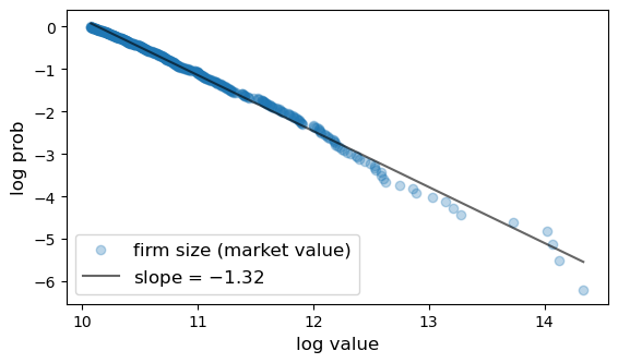
Largest 500 firms in 2020 taken from Forbes Global 2000
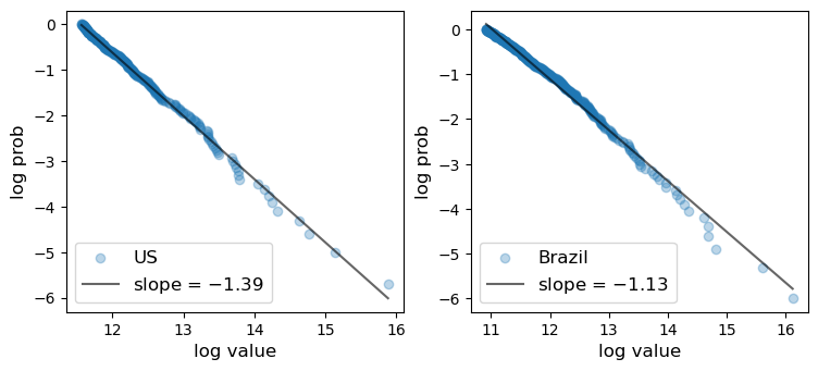
City Sizes in the US and Brazil
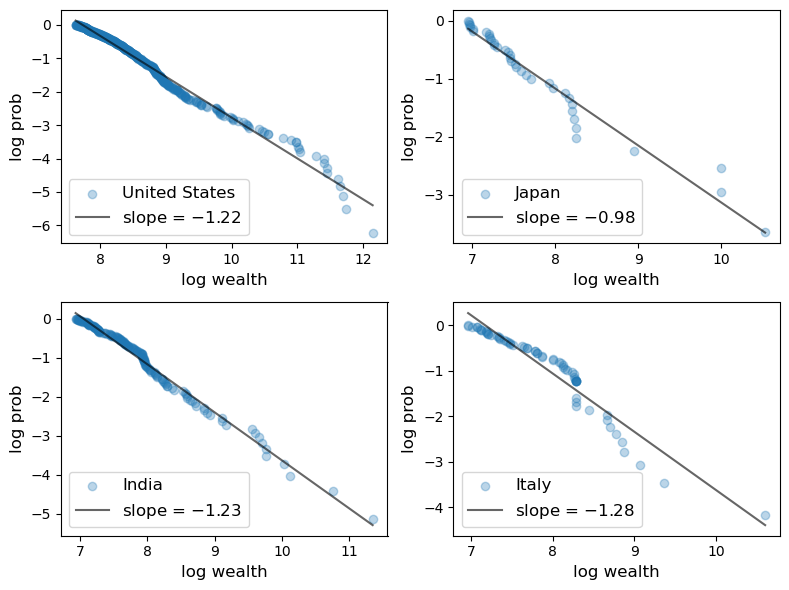
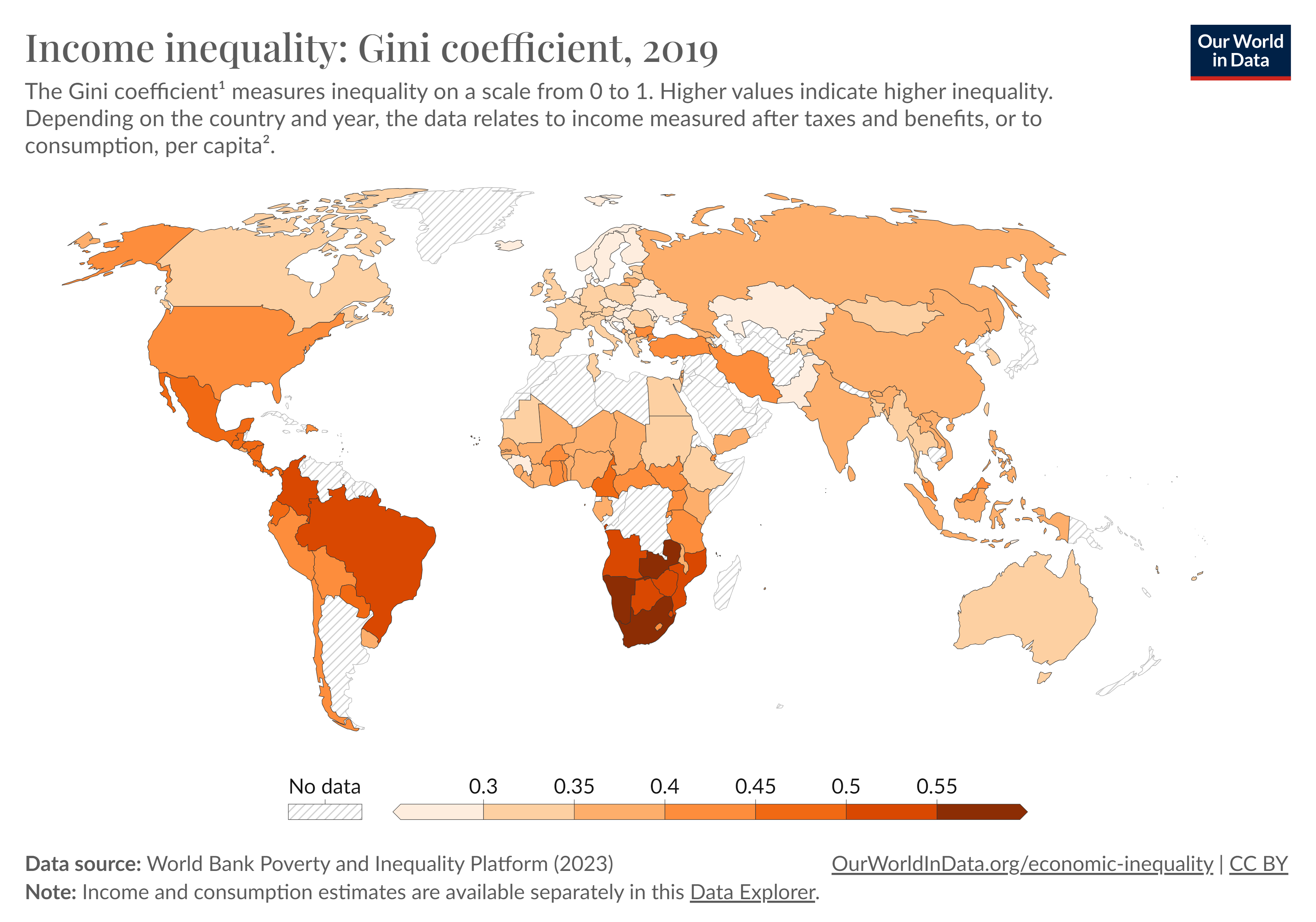
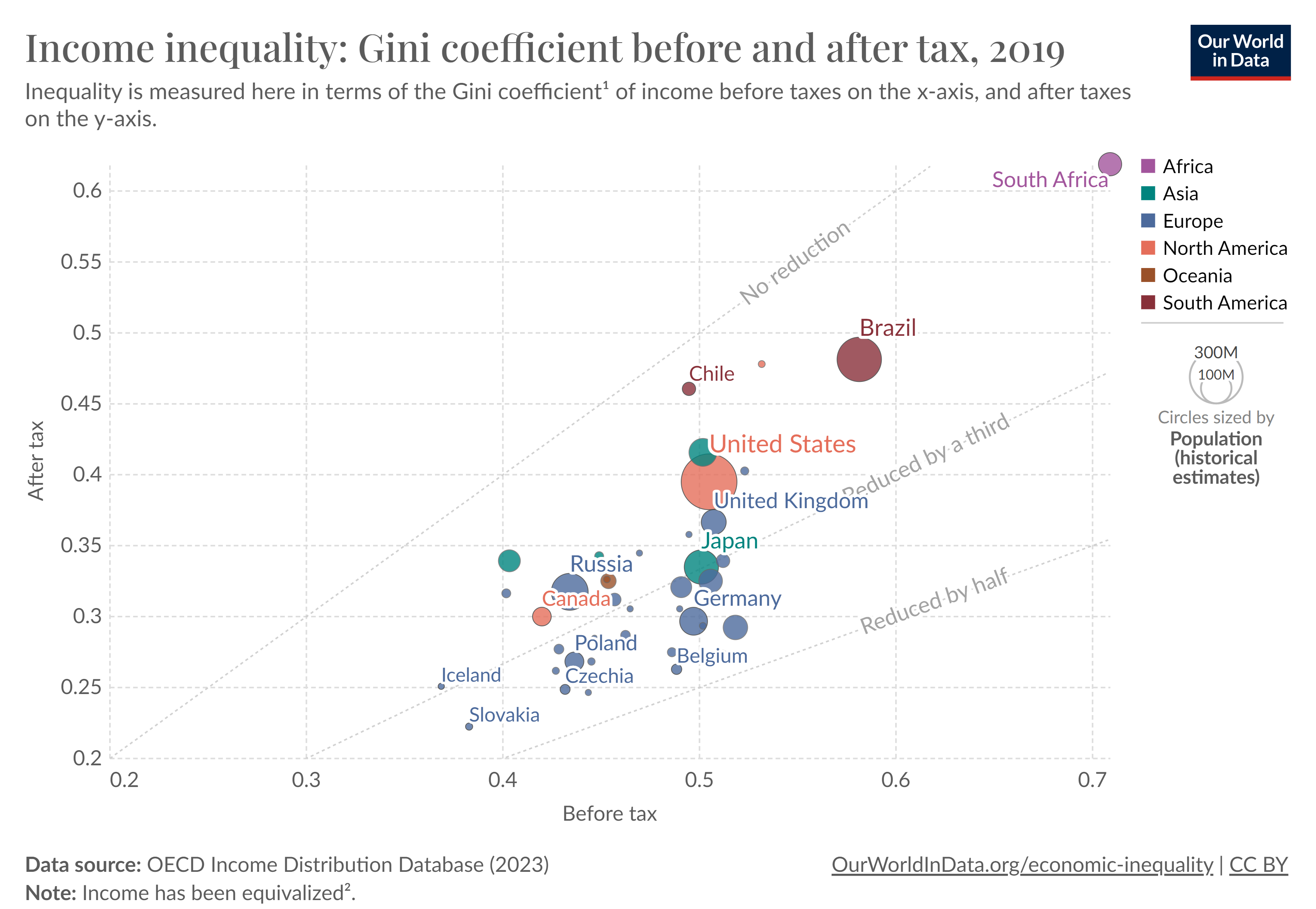
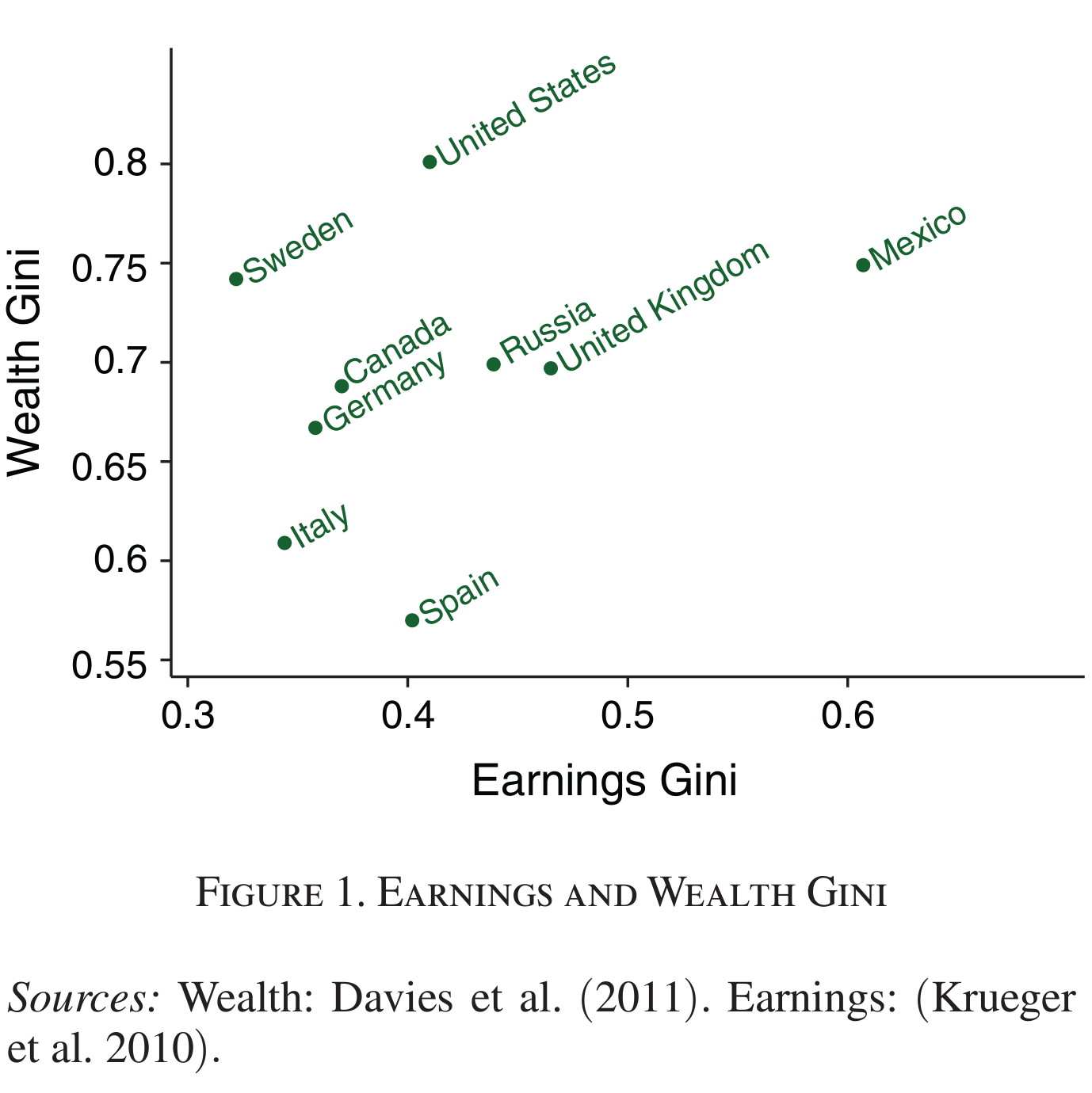
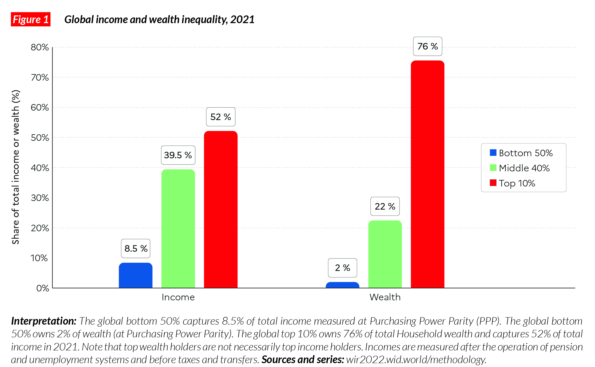
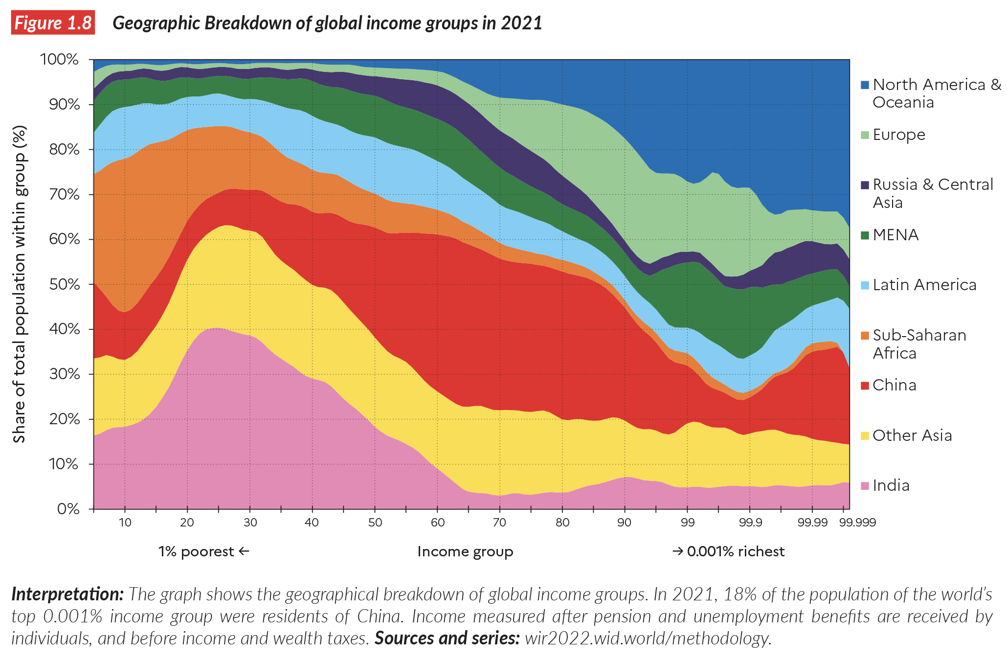
Wealth Distribution Across Countries
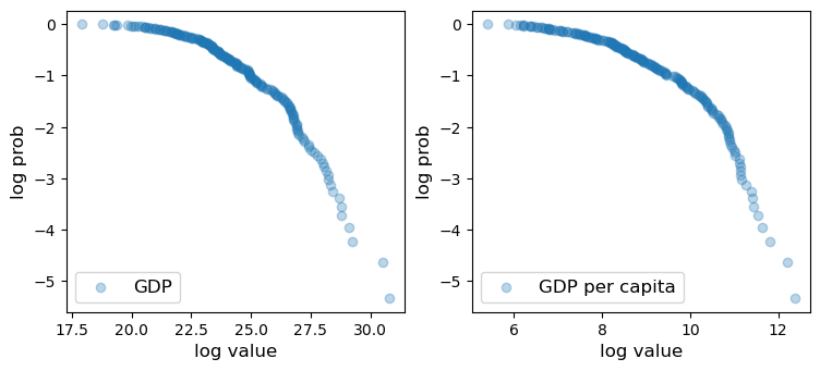
GDP Across Countries
Zipf Distribution? \(\alpha = 1.059\)
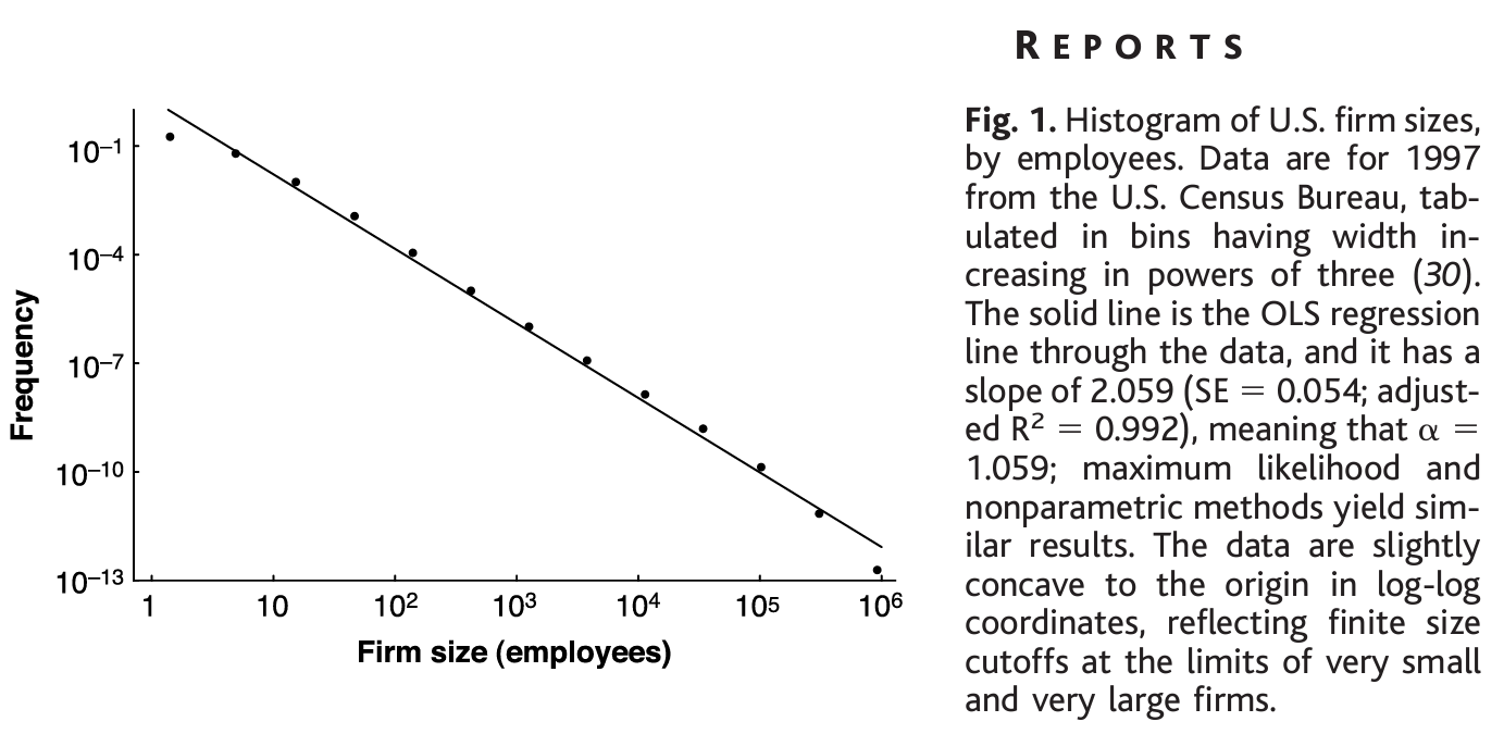
See https://www.science.org/doi/10.1126/science.1062081 by Axtell
Simulation of a Process for Growth

Log-Log Plot
X_T = sort(X[:, end])
x_T = log.(X_T)
F_T = (1:length(X_T)) / length(X_T)
y_T = log.(1 .- F_T)
(;a, b) = simple_regression(x_T[1:end-1],
                            y_T[1:end-1])
plot(x_T, y_T; label = L"\log(1-F(X))",
     xlabel=L"\log(X)", size = (600, 400))
a_r = round(a, digits = 2)
plot!(x_T, a*x_T .+ b;
      label = L"a=%$a_r", style = :dash)
Implementation

With Cruder Samples Still Fairly Smooth

Lorenz Curve for Pareto

Calculation and Comparison to Theoretical

From From Benhabib, Bisin, Luo
Example Simulation

Lorenz Curves and Returns on Wealth

Gini Coefficients

Lorenz Curves and Volatility

