Course Overview and Computational Environment
Undergraduate Computational Macro
Course Overview and Objectives
Course Structure and Prerequisites
“Macroeconomics on a computer”
- mostly macro-finance + macro-labor
Focus: math + theory + computation
- Not an intro programming course
- Not a data science or econometrics course
Goal: build structural models for conducting counterfactuals
- lots of simulation
- little data / empirics
Complements “field” and applied courses
- empirics, estimation, inference, data science
- e.g., which regression makes sense to run, how to interpret, etc.
Prerequisites
Required courses (choose one from each group)
- ECON 301, ECON 302, ECON 304, ECON 315, COMM 295, FRE 295
- ECON 323, CPSC 103, CPSC 107, CPSC 110, CPSC 301, MATH 210, COMM 337, PHYS 210, EOSC 211, APSC 160
- MATH 152, MATH 221, MATH 223
Note that micro, not macro, is a requirement
Formal programming course in a general-purpose language
- Stata and R don’t count
- self-study isn’t enough
Math background: talk to me if unsure
- ECON 307 or significant linear algebra in a different course can substitute
Assessments
- Grading:
- 6-8 problem sets: 15% (total)
- Midterm exam: 30%
- Final exam: 50%
- Participation: 5%
- Problem sets will be crucial for studying for exams
- The midterm and final examinations may be done in a computer lab, on your own computer in class, or on paper
- Decision will be made later in term, depending on lab availability.
- Not testing programming skills
- Problem sets will start off short and easy to help those with less programming experience, and then build in (economics) complexity.
Course Policies
Please see the syllabus for details on
- Collaboration policy
- AI policy
- Academic integrity, etc.
Note the policy on accommodations
- Email me about non-exam accommodations (e.g., late problem sets)
- Exam accommodations follow the listed process
- The midterm dates will be announced in the first week of class
- There are no make-up or deferred exams. I get to choose the alternative (e.g., changing weight on exams, oral exam)
Exam Accommodations
- Students sometimes get sick right before exams and worry about whether accommodations are possible
- The university typically grants accommodations unless there is a clear pattern of behavior
- If you are sick before an exam and email me last minute, assume an accommodation will happen (unless you have a history)
- Don’t panic! Go back to bed
- Missing the midterm makes accommodations for the final more difficult
- In those cases, a late withdrawal is more likely than a final-exam accommodation
Programming Languages
Which Language?
Econ/finance uses many languages
- Matlab, Python, Julia, Fortran, C++, Stata, Dynare, R, Stan, …
Trade-offs everywhere
- each is strong for some tasks, weak for others
- some are specialized (e.g. Stata, R)
My view: learn at least two general-purpose languages
- it will pay off over your career
Results from 2025 Survey
- Surveys conducted at the end of the term.
- Allows students time to reflect on the long-term benefits of the toolchain versus the initial learning curve.
Julia vs. Python Preference
Question: Given the trade-offs discussed in class (speed/verbosity), which do you prefer for this course?
| Preference | Percentage |
|---|---|
| Strongly prefer Julia | 44% |
| Weakly prefer Julia | 28% |
| Indifferent | 11% |
| Weakly prefer Python | 6% |
| Strongly prefer Python | 11% |
Exam Format Preference
Question: Preference between computer-lab based coding exams vs. traditional paper-based exams.
| Preference | Percentage |
|---|---|
| Strongly prefer coding-based | 44% |
| Weakly prefer coding-based | 28% |
| Indifferent | 6% |
| Weakly prefer paper-based | 17% |
| Strongly prefer paper-based | 6% |
Coding Difficulty on Exams
Question: Assessment of the amount and difficulty of writing code during the exams.
| Difficulty Level | Percentage |
|---|---|
| Very easy | 28% |
| Relatively easy | 39% |
| Medium | 22% |
| Fairly hard | 11% |
Why Learn Multiple Languages
- Languages come and go; skills compound
- Second language → better programmer
- Third language → much easier
- Everyone claims they know Python on job and grad school applications
- Another language = differentiation
- Signals computational maturity
- Julia works well for this and is more directly useful in this domain than alternatives (e.g., Rust, C++)
Why Julia for Economics and Finance
- Python: great for data + ML and linear-algebra heavy tasks
- Verbose for math and high-performance simulation
- Performance needs frameworks (e.g., JAX) or C/C++
- Python + (JAX, Pytorch, …):
- Many frameworks exist, but code for this course would be more complex
- Often work great if problem maps well into ML-style “kernels”, but tricky for more general problems
- Julia: designed for math and scientific computing
- Natural for linear algebra and dynamics
- Fast without leaving the language
- Widely used in econ & finance research
Don’t Worry If You’re New to Programming
- Marginal cost of learning a new language decreases with each new language
- High transferability of programming concepts
- Julia follows naturally from the prereqs
- Prior formal course in Matlab or Python
- R is not sufficient preparation
- Submissions must be in Julia
Quantitative, Empirical, and Theoretical Economics
Why Isn’t “Big Data”/ML/Statistics Enough?
Economists asked this long before “big data”
Statistics works only if you already have the right model for the experiment
Historical data rarely has variation in crucial directions
- policies don’t change at random
- many counterfactuals were never tried
Why Macro Is Especially Hard
Dynamics + expectations: choices today depend on forecasts about tomorrow
General equilibrium: policy shifts prices, constraints, and behavior together
People adapt when public policy or prices change
- incentives shift
- beliefs and forecasts shift
Canonical warnings
- Cowles Commission
- Lucas Critique
- Policy Ineffectiveness (Sargent–Wallace)
- Time Inconsistency (Kydland–Prescott)
More data or fancier estimators can’t fix the wrong “model”
Forecasts, Distributions, and DGPs
In stats/ML/econometrics we start with a Data Generating Process (DGP)
In macro the hard part is: which DGP lets us answer a particular question?
Think probabilistically: the economy is a joint distribution over
- observables (data)
- unobserved (e.g., latent) states
- shocks
- “deep” parameters (e.g., preferences, technology)
Different assumptions \(\Rightarrow\) different “experiments,” even with the same dataset
Joint distributions let you ask conditional questions
- forecasts: “what is likely next?”
- policy: “what changes if we intervene?”
- distributional: “who gains/loses?”
Counterfactuals: “What If?”
Most interesting problems in economics are counterfactuals
- What would unemployment have been if the government had not intervened during the recession?
- What would have been her income if she had not gone to college, or if she wasn’t subjected to gender bias?
By definition these are not observable. If we had the data already we wouldn’t need to ponder these “What if?” questions
How can you answer a question with data that doesn’t exist?
Theory and Structural Models
To answer “what if?”, you need a disciplined way to “make something up”
Theory is what turns data into a model of the economy
A model is a structured joint distribution
- behavior + constraints + market clearing
- plus shocks and expectations
This structure constrains counterfactuals
- what can change when policy/prices move
- what cannot be held fixed (endogenous objects)
Approach in this Course
Counterfactuals are not in the data \(\Rightarrow\) you need assumptions
Three complementary approaches
- Structural models: theory + equilibrium + dynamics
- Causal inference: identification via independence/exogeneity assumptions
- Randomized experiments: treatment variation by design
This course: simulations + structural models
- “quantitative economics”
Macroeconomic Models Require Lots of Tools
Macro counterfactuals are hard because
- decisions are dynamic and stochastic
- agents are forward-looking
- prices/markets create general equilibrium feedback
- heterogeneity makes distributions central
- policy changes behavior (and expectations) over time
We can write the math down to “keep us honest”
In macro, we often can’t solve important problems analytically
- need computational tools to simulate and solve models
Tools Topics
See Syllabus for more details
- Linear algebra and basic scientific computing
- Geometric Series and Discrete Time Dynamics
- Basic Stochastic Processes
- Linear State Space Models
- Markov Chains
- Dynamic Programming
Applications Topics
The tools are interleaved with applications such as
- Marginal Propensity to Consume
- Dynamics of Wealth and Distributions
- Permanent Income Model
- Models of Unemployment
- Asset Pricing
- Lucas Trees and No-arbitrage Option Pricing
- Recursive Equilibria and the McCall Search Model
- Time permitting: Rational Expectations and Firm Equilibria, Growth Models
Computational Environment
Setup
- You can install Julia on your laptop by following these instructions
- While one can use Julia entirely from just Jupyter notebooks, we will introduce basic GitHub and VS Code usage as well to help broaden your exposure to computational tools.
- Apply for academic pack and activate GitHub Copilot Pro
- No need to install conda/jupyter/etc. unless you prefer it.
- So my suggestion is to challenge yourself to learn VS Code, GitHub, and other tools. Further signalling for RA/predoc/jobs/etc.
Summary of Installation
- Install Git
- Install VS Code
- Install Julia following the Juliaup instructions
- Windows:
winget install julia -s msstorein a terminal - Linux/Mac:
curl -fsSL https://install.julialang.org | shin a terminal
- Windows:
- Install the VS Code Julia extension
- Clone the notebooks repository and install packages (crucial! see next slide)
Clone Notebooks and Install Packages
Open the command palette with
<Ctrl+Shift+P>or<Cmd+Shift+P>on mac and type> Git: Cloneand choosehttps://github.com/jlperla/undergrad_computational_macro_notebooksStart a terminal with
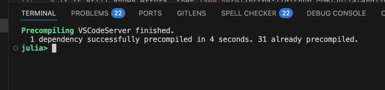
<Ctrl+Shift+P>or<Cmd+Shift+P>on mac and type> Julia: Start REPL- The first time you run this, it will say it is
precompiling VSCodeServer
- The first time you run this, it will say it is
Instantiate packages by running VS Code terminal
] instantiate, where]enters package mode- This will usually take 5-10 minutes to precompile and install the first time
- If there are any errors please email the log to us
Then use VS Code to open any of the notebooks in that folder
Troubleshooting
VS Code Extension Screenshots
First REPL should look like this:
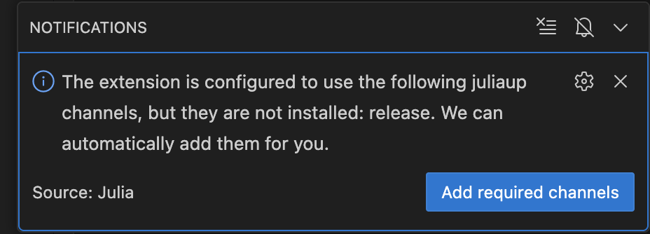
Update juliaup release channel? Yes:
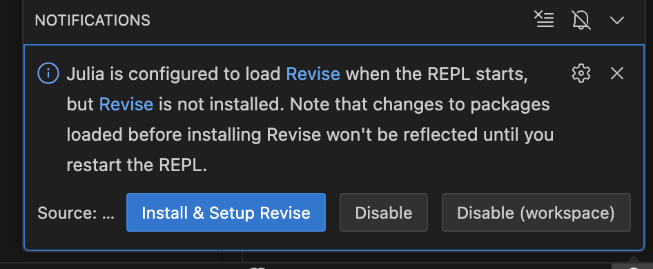
Install Revise? Your choice, but restart VS Code after installation:
If you…
- do not see the
] instantiatesetup install a bunch of pacakges, you likely didn’t start the Julia REPL in the VS Code terminal- If you aren’t using VS Code, then make sure to start julia with
julia --projectin the notebooks repo
- If you aren’t using VS Code, then make sure to start julia with
- get an error when you run a notebook that a package not being installed, you likely forgot the
] instantiatestep - see
Failed to precompile...then there is likely a problem. Send us the text - get errors that it can’t find
juliathen restart your terminals, vscode, etc. to ensure environment variables are applied- if you still have problems, then you likely didn’t follow the
juliaupinstructions for adding something to an environment variable
- if you still have problems, then you likely didn’t follow the
Precompile errors
- If you see errors like the following, ignore, restart your VS Code and REPL, and try
] instantiateagain
SYSTEM: caught exception of type :MethodError while trying to print a failed Task notice; giving up
MethodError: no method matching pipe_writer(::VSCodeServer.IJuliaCore.IJuliaStdio{Base.PipeEndpoint, typeof(VSCodeServer.io_send_callback)})
The applicable method may be too new: running in world age 38658, while current world is 38713.

Closest candidates are:
  pipe_writer(::VSCodeServer.IJuliaCore.IJuliaStdio) (method too new to be called from this world context.)
   @ VSCodeServer ~/.vscode/extensions/julialang.language-julia-1.173.2/scripts/packages/IJuliaCore/src/stdio.jl:16
  pipe_writer(!Matched::Base.Process)
   @ Base process.jl:23
  pipe_writer(!Matched::Base.AnnotatedIOBuffer)
   @ Base strings/annotated_io.jl:21
Some Common Errors on MacOS/Linux
To open a terminal on MacOS
- Press
Cmd + Spaceto open Spotlight, then typeTerminal - Or with VS Code
<Cmd-Shift-P>thenView: Toggle Terminal
- Press
If you get permissions problems try
sudo curl -fsSL https://install.julialang.org | shIf it still shows errors, then see here and do some combo of
sudo chown $(id -u):$(id -g) ~/.bashrc sudo chown $(id -u):$(id -g) ~/.zshrc sudo chown $(id -u):$(id -g) ~/.bash_profile- Then retry
sudo curl -fsSL https://install.julialang.org | sh
- Then retry
Resetting
Uninstall the Julia extension in VS Code to be safe
Then close VS Code and any Julia terminals
Then delete the
.juliafolder in your home directory- On MacOS/Linux, open a terminal and delete the whole
.juliafolder with
rm -rf ~/.julia- On Windows, the folder is usually in
C:\Users\YourUsername\.julia
- On MacOS/Linux, open a terminal and delete the whole
Open up VS Code and reinstall the Julia extension
Follow the instructions to open a Julia REPL in VS Code and install the packages
Pulling Notebook Updates
- As changes are made in the notebook repository, you will want to pull the latest changes
- Make sure to backup any of the notebooks first (especially any modified problem sets to ensure they are not lost)
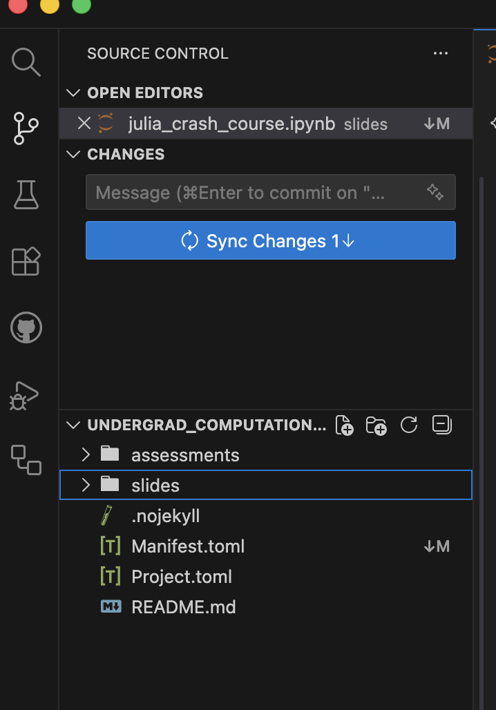
- The folder in VS Code, it should show a notification in the bottom left corner, or when you click on the “Source Control” icon on the left sidebar
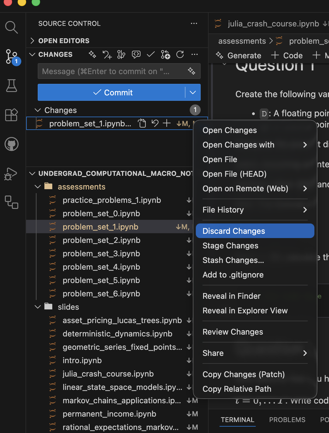
Discarding Local Changes
- If you have made local changes,can discard if they clash with upstream changes.
- Remember to backup any modified problem sets first!
- Click “Source Control” icon, right-click changed files, choose “Discard Changes”
- If
Manifest.tomlchanged, this is especially important - Re-run
] instantiateafter pulling
Environments
Julia Environment Basics
- Project files keep track of dependencies and make things reproducible
- Similar to Python’s virtual environments but easier to use
- VS Code and Jupyter will automatically activate a
Project.toml- In REPL or Jupyter enter
]for managing packages - Can manually activate with
] activateor] activate path/to/project - On commandline, can use
julia --project
- In REPL or Jupyter enter
- With activated project, use
] instantiateto install all the packages - For this course: no package management required after instantiation
Reproducibility
- ALWAYS use a
Project.tomlfile- Keep your global environment as clean
- Associated with
Project.tomlis aManifest.tomlfile which establishes the exact versions for reproducibility] instantiatewill install the exact versions- Less important for us, but very useful for reproducibility in research to distribute with project