Ensure you modify the field above with your name and student number above immediately
The exam has XXXXX questions, each with multiple parts for a total of XXXXX points. You may not finish the exam, so best to do your best answering all questions to the extent possible and not get stuck on any one question.
This exam is closed book and accessing the internet is not permitted
See the formula “sheet” embedded at the end of this notebook for reference
You can the internal help as required (see the Jupyterhub menu, use Settings/Show Contextual Help)
Execute the file to begin, which will also check your setup. To do this in Jupyter, in the menu go > Run > Run All Cells or the equivalent buttons
Edit this file directly, and in-place as an ipynb file, which we will automatically download at the end of the exam time directly. In particular
DO NOT rename this file with your name. It is automatically associated with your canvas account
DO NOT save-as the file, move it, or export to pdf or html
DO NOT add any additional packages
Save the notebook as you are working
We will only grade what is saved at the end of the exam in this exact file, and it is your responsibility to ensure the file is saved
We will not execute the notebook, so ensure all code, figures, etc. are ready as-is upon saving for submission
Ensure you edit the results in the code blocks or markup blocks indicated as we will not grade anything outside of those
You will not be judged on code quality directly, but code clarity may be required for us to ensure you understood the problem directly
If a question requires math, you can try to put latex inside of the cells but will not be judged on whether you write latex vs. math in text that doesn’t quite match latex. But it should be clear
# Packages available# DO NOT MODIFY OR ADD PACKAGESusingDistributions, Plots, LaTeXStrings, LinearAlgebra, Statistics, Random
Precompiling packages...
    980.0 ms  ✓ StatsAPI
   1330.8 ms  ✓ Statistics
   1897.1 ms  ✓ FillArrays
   1016.4 ms  ✓ Reexport
   1362.9 ms  ✓ DocStringExtensions
   1092.3 ms  ✓ PtrArrays
   3866.1 ms  ✓ OrderedCollections
   1045.1 ms  ✓ DataAPI
   1754.1 ms  ✓ PDMats
   1282.7 ms  ✓ Preferences
   1036.3 ms  ✓ FillArrays → FillArraysStatisticsExt
   1340.3 ms  ✓ Statistics → SparseArraysExt
   6090.4 ms  ✓ IrrationalConstants
   1599.6 ms  ✓ FillArrays → FillArraysSparseArraysExt
   1431.6 ms  ✓ AliasTables
   1495.6 ms  ✓ FillArrays → FillArraysPDMatsExt
   3158.4 ms  ✓ DataStructures
   1220.9 ms  ✓ JLLWrappers
   1261.2 ms  ✓ LogExpFunctions
   4021.1 ms  ✓ Missings
   1288.6 ms  ✓ SortingAlgorithms
   1397.6 ms  ✓ Rmath_jll
   1467.3 ms  ✓ OpenSpecFun_jll
   1606.2 ms  ✓ Rmath
   4905.6 ms  ✓ QuadGK
   5811.3 ms  ✓ StatsBase
   4217.6 ms  ✓ SpecialFunctions
    922.3 ms  ✓ PDMats → StatsBaseExt
   1187.9 ms  ✓ HypergeometricFunctions
   2637.1 ms  ✓ StatsFuns
   4749.0 ms  ✓ Distributions
  31 dependencies successfully precompiled in 29 seconds. 10 already precompiled.
Precompiling packages...
    913.3 ms  ✓ TensorCore
    928.9 ms  ✓ Contour
   1186.2 ms  ✓ LaTeXStrings
   1359.9 ms  ✓ Measures
   3134.9 ms  ✓ Format
   2188.6 ms  ✓ Requires
   1038.6 ms  ✓ StableRNGs
   5683.0 ms  ✓ Grisu
   8064.6 ms  ✓ MacroTools
   1523.4 ms  ✓ URIs
   1056.3 ms  ✓ SimpleBufferStream
   1379.1 ms  ✓ TranscodingStreams
   4374.6 ms  ✓ Unzip
   1020.0 ms  ✓ DelimitedFiles
   1017.9 ms  ✓ BitFlags
   3515.0 ms  ✓ NaNMath
   2347.6 ms  ✓ ConcurrentUtilities
   1210.7 ms  ✓ LoggingExtras
   1385.1 ms  ✓ PrecompileTools
   4121.7 ms  ✓ StructUtils
   1011.9 ms  ✓ ExceptionUnwrapping
   2704.9 ms  ✓ UnicodeFun
   1668.6 ms  ✓ Graphite2_jll
   1241.4 ms  ✓ Libmount_jll
   1149.6 ms  ✓ EpollShim_jll
   1881.3 ms  ✓ LLVMOpenMP_jll
  10049.8 ms  ✓ FixedPointNumbers
   1289.2 ms  ✓ Bzip2_jll
   1372.0 ms  ✓ Xorg_libXau_jll
   1595.3 ms  ✓ Xorg_libICE_jll
   1623.0 ms  ✓ libpng_jll
   1682.9 ms  ✓ libfdk_aac_jll
   1268.3 ms  ✓ LERC_jll
   1948.2 ms  ✓ LAME_jll
   1517.0 ms  ✓ fzf_jll
   1919.5 ms  ✓ JpegTurbo_jll
   1659.9 ms  ✓ XZ_jll
   1544.8 ms  ✓ Ogg_jll
   1368.2 ms  ✓ mtdev_jll
   1883.6 ms  ✓ Xorg_libXdmcp_jll
   1404.3 ms  ✓ x265_jll
   1646.6 ms  ✓ x264_jll
   1385.1 ms  ✓ libaom_jll
   1820.7 ms  ✓ MbedTLS_jll
   1425.1 ms  ✓ Zstd_jll
   1957.6 ms  ✓ Expat_jll
   1289.6 ms  ✓ LZO_jll
   1399.3 ms  ✓ Opus_jll
   1352.0 ms  ✓ Xorg_xtrans_jll
   1770.5 ms  ✓ libevdev_jll
   1829.2 ms  ✓ Libiconv_jll
   1192.1 ms  ✓ Libffi_jll
   1687.8 ms  ✓ eudev_jll
   1399.3 ms  ✓ FriBidi_jll
   1589.6 ms  ✓ Libuuid_jll
   1148.3 ms  ✓ Showoff
   1353.6 ms  ✓ CodecZlib
   4746.2 ms  ✓ OpenSSL
   4380.1 ms  ✓ RecipesBase
   1665.8 ms  ✓ Pixman_jll
   1826.7 ms  ✓ FreeType2_jll
   1482.6 ms  ✓ Xorg_libSM_jll
   5122.6 ms  ✓ ColorTypes
   1822.0 ms  ✓ JLFzf
   1618.4 ms  ✓ libvorbis_jll
   3049.7 ms  ✓ Ghostscript_jll
   2983.7 ms  ✓ MbedTLS
   4326.0 ms  ✓ Xorg_libxcb_jll
   1725.2 ms  ✓ Libtiff_jll
   1289.8 ms  ✓ Dbus_jll
   1764.3 ms  ✓ GettextRuntime_jll
   1986.1 ms  ✓ Wayland_jll
   1142.9 ms  ✓ libinput_jll
   2183.9 ms  ✓ Fontconfig_jll
    994.3 ms  ✓ ColorTypes → StyledStringsExt
   7131.3 ms  ✓ ColorVectorSpace
  13003.7 ms  ✓ Colors
  10537.8 ms  ✓ Latexify
   1158.2 ms  ✓ Xorg_xcb_util_jll
   1443.3 ms  ✓ Xorg_libX11_jll
   1666.0 ms  ✓ Glib_jll
  42836.8 ms  ✓ Parsers
   1774.8 ms  ✓ Latexify → SparseArraysExt
   1552.3 ms  ✓ Xorg_xcb_util_image_jll
   1994.8 ms  ✓ Xorg_xcb_util_keysyms_jll
   1571.8 ms  ✓ Xorg_xcb_util_renderutil_jll
   8960.0 ms  ✓ ColorSchemes
   1347.2 ms  ✓ Xorg_xcb_util_wm_jll
   1528.6 ms  ✓ Xorg_libXrender_jll
   1200.3 ms  ✓ Xorg_libXext_jll
   1234.1 ms  ✓ Xorg_libXfixes_jll
   1842.0 ms  ✓ Xorg_libxkbfile_jll
   1807.6 ms  ✓ Xorg_xcb_util_cursor_jll
  12502.3 ms  ✓ JSON
   1732.9 ms  ✓ Xorg_libXinerama_jll
   1782.6 ms  ✓ Xorg_libXrandr_jll
   2267.9 ms  ✓ Libglvnd_jll
   2064.3 ms  ✓ Cairo_jll
   1066.0 ms  ✓ Xorg_libXcursor_jll
   1768.2 ms  ✓ Xorg_libXi_jll
   1897.9 ms  ✓ Xorg_xkbcomp_jll
   1962.7 ms  ✓ HarfBuzz_jll
   1529.7 ms  ✓ Xorg_xkeyboard_config_jll
   1496.2 ms  ✓ libass_jll
   2040.7 ms  ✓ Pango_jll
  30642.1 ms  ✓ PlotUtils
   1804.7 ms  ✓ xkbcommon_jll
   2310.1 ms  ✓ FFMPEG_jll
  56360.7 ms  ✓ HTTP
   1820.2 ms  ✓ Vulkan_Loader_jll
   7445.4 ms  ✓ PlotThemes
   1636.5 ms  ✓ libdecor_jll
   1561.3 ms  ✓ FFMPEG
   2866.5 ms  ✓ Qt6Base_jll
   2094.5 ms  ✓ GLFW_jll
   1654.2 ms  ✓ Qt6ShaderTools_jll
   2060.1 ms  ✓ GR_jll
  12913.7 ms  ✓ RecipesPipeline
   3407.6 ms  ✓ Qt6Declarative_jll
    769.1 ms  ✓ Qt6Wayland_jll
   5191.7 ms  ✓ GR
  82652.3 ms  ✓ Plots
  122 dependencies successfully precompiled in 231 seconds. 55 already precompiled.
Precompiling packages...
    696.4 ms  ✓ ColorVectorSpace → SpecialFunctionsExt
  1 dependency successfully precompiled in 1 seconds. 20 already precompiled.
Precompiling packages...
   1261.6 ms  ✓ QuartoNotebookWorkerJSONExt (serial)
  1 dependency successfully precompiled in 1 seconds
Precompiling packages...
   2616.8 ms  ✓ QuartoNotebookWorkerPlotsExt (serial)
  1 dependency successfully precompiled in 3 seconds
Precompiling packages...
   1013.5 ms  ✓ QuartoNotebookWorkerLaTeXStringsExt (serial)
  1 dependency successfully precompiled in 1 seconds
Take the following functions from our previous lectures
# DO NOT MODIFYfunctionlorenz(v) # assumed sorted vector S =cumsum(v) # cumulative sums: [v[1], v[1] + v[2], ... ] F = (1:length(v)) /length(v) L = S ./ S[end]return (; F, L) # returns named tupleend# Assumes that v is sorted!gini(v) = (2*sum(i * y for (i,y) inenumerate(v))/sum(v)- (length(v) +1))/length(v)functionsimple_regression(x, y) x_bar =mean(x) y_bar =mean(y) a =sum((x .- x_bar).*(y .- y_bar)) /sum((x .- x_bar).^2) b = y_bar - a * x_barreturn (;a, b)end
simple_regression (generic function with 1 method)
Short Question 1
With a CDF of a distribution \(F(x)\) with an accompanying counter-cdf \(1-F(x)\), what is the definition of a power-law tail? For a stochastic process \(X_t\), what features of that stochastic process might lead to a power-law tail in the stationary distribution?
Answer:
(double click to edit your answer)
Short Question 2
If you are trying to understand wealth inequality, what features of the distribution are ideal to examine using (a) Lorenz Curves; (b) Gini Coefficients; and (c) Power Law Tails
Answer:
(double click to edit your answer)
Short Question 3
If I calculate a log-log plot of a distribution to examine whether it has heavy tails, what should I plot for the x-axis and y-axis? If I did a linear regression and found that the slope was -2, would that necessarily say that the distribution was a power-law distribution? Why or why not?
Answer:
(double click to edit your answer)
Short Question 4
If a log-log plot showed a slope of -1.5 with a clear linear relationship in the right tail, what is the implied power-law exponent? What does this tell us about moments of the underlying distribution?
Answer:
(double click to edit your answer)
Short Question 5
Compare stochastic processes:
\(X_{t+1} = a_{t+1} X_t + b\)
\(X_{t+1} = X_t + a_{t+1} + b\)
where in both cases \(a_{t+1}\) are IID shocks. Which stochastic process would you expect may have power-law tails in their stationary distribution, and why? What if \(b = 0\) in both cases? Provide intuition for the differences.
Answer:
(double click to edit your answer)
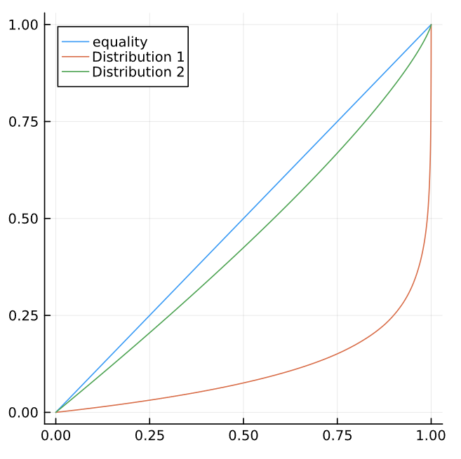
Short Question 6
Take the following figure showing the Lorenz Curves for data from two different distributions. What can you infer about the inequality in the two distributions? Roughly what would you expect the Gini coefficients to be for the two distributions?
Answer:
(double click to edit your answer)
Short Question 7
Given a mapping \(F : \mathbb{R}^N \to \mathbb{R}^N\) what is the definition of a fixed point \(x^*\) of this mapping? Does it always exist? If it exists, is it unique?
Answer:
(double click to edit your answer)
Short Question 8
Explain the importance of the fixed factor of production, land, in the Malthusian growth model
Answer:
(double click to edit your answer)
Short Question 9
An asset pays off a deterministic stream of income, \(\{y_{t+j}\}_{j=0}^{\infty}\), and a risk-neutral agent prices this using a discount factor \(0 < \beta < 1\). The PDV of the income is then \(p_t = \sum_{j = 0}^{\infty}\beta^j y_{t+j}\) The agent prices this asset using the recursive formulation
\[
p_t = y_t + \beta p_{t+1}
\]
Briefly interpret this recursive equation from the agent’s perspective.
Answer:
(double click to edit your answer)
Short Question 10
What is a state space model? Explain what type of problem a Kalman Filter solves. What are the key assumptions on the stochastic processes, priors, etc. that make it applicable?
Answer:
(double click to edit your answer)
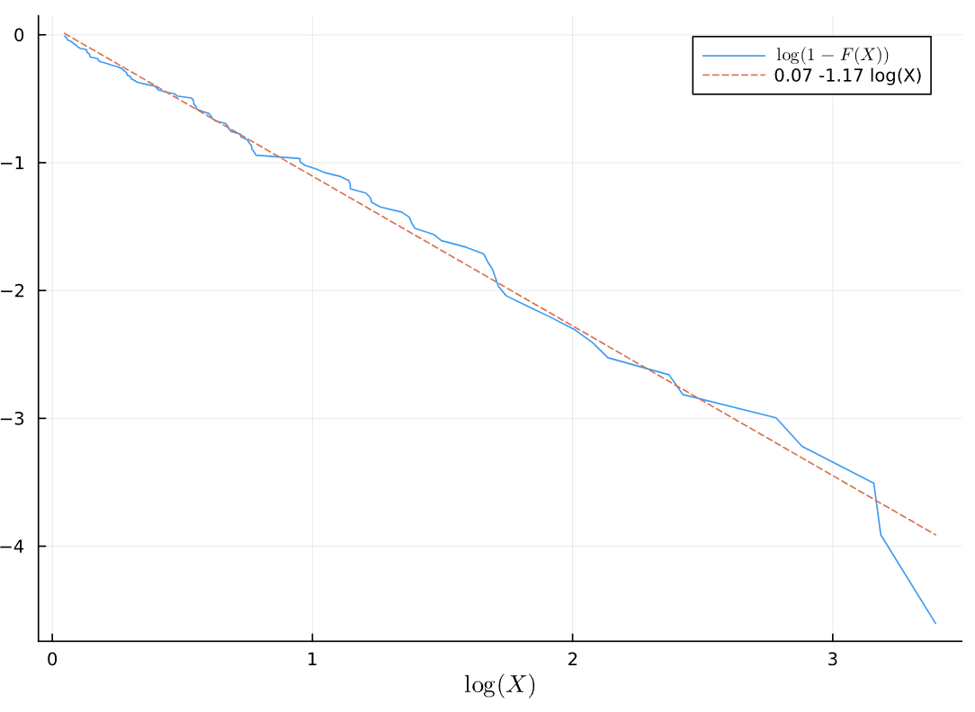
Question 0
Consider for some \(X_t \sim F\) IID draws from a distribution the log-log plot using the empirical CDF. The dotted line plots the linear regression with this data, with the intercept and slope shown on the legend.
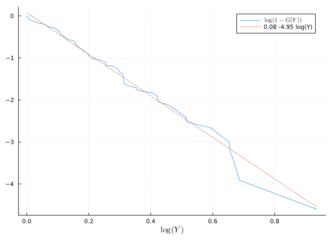
Consider the log-log plot of 100 IID draws from a different distribution \(Y_t \sim F\).
Compare the \(X_t\) and \(Y_t\) log-log plots. What can you infer about these distributions?
Answer:
(double click to edit your answer)
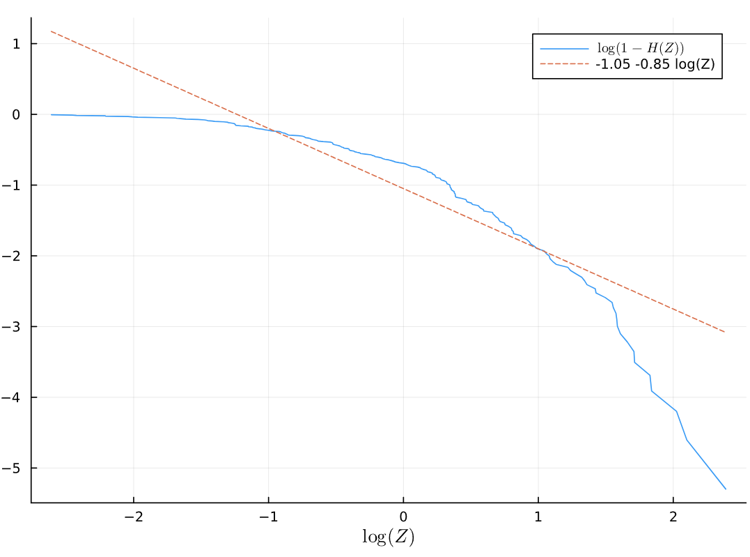
Now consider the log-log plot of draws from a third distribution \(Z_t \sim F\)
The log-log plot of the \(Z_t\) draws
What can you infer about this distribution compared to the other two?
Answer:
(double click to edit your answer)
Question 1
Following the notes on AR(1) processes rather than plotting the distribution as normal instead lets see what the stationary distribution looks like with simulation.
Part (a)
From \(X_0 = 1.0\) simulate up to \(T=2000\) using the process
\[
X_t = a X_{t-1} + b + c W_t
\]
Where \(a=0.98, b=0.1, c=0.02\).
T =2000X_0 =1.0a =0.98b =0.1c =0.02# Add code here
0.02
Part (b)
On the same graph plot the histogram of those simulated values (i.e., \(\{X_0, \ldots X_T\}\)) then plot the density of the stationary distribution calculated in closed form in those notes (i.e. create a normal distribution with \(\mu^* = b/(1-a)\) and \(v^* = c^2/(1 - a^2)\)
Hint: histogram(X, normed=true) normalizes the empirical draws so they are a proper PMF.
# Add code here
Part (c)
Now, do the same plot using the 10th to 500th observations (i.e., \(\{X_{10}, \ldots X_{500}\}\))
# Add code here
And then a separate plot using the rest
# Add code here
Compare how these line up? Explain why each is better or worse?
Answer:
(double click to edit your answer)
Part (d)
Change the c parameter to be 0.2.
Now repeat the display of the two histograms (1) split of the 10th to 500th ; and (2) the remainder
T =2000X_0 =1.0a =0.98b =0.1c =0.2# Add code here, creating new cells as required
0.2
Compare this to part (c)? Have the results changed and if so, then why?
Answer:
(double click to edit your answer)
Question 2
In this problem we will examine wealth dynamics for a simpler setup. Log income, \(\log y_t\) follows an AR(1) process,
where \(\epsilon_{1,t+1} \sim N(0,1)\) and \(\epsilon_{2,t+1} \sim N(0,1)\) are IID shocks.
As in the wealth dynamics problem from before, the evolution of wealth is given by
\[
w_{t+1} = R_{t+1}s(w_t) + y_{t+1}
\]
where \(s(w_t)\) is the exogenously given savings function from before,
\[
s(w) = s_0 w \cdot \mathbb 1\{w \geq \hat w\} = \begin{cases} s_0 w & w \geq \hat{w}\\
0 & w < \hat{w}
\end{cases}
\]
For a constant \(s_0 \in (0,1)\) which is savings rate and \(\hat{w}\geq 0\) is a minimum wealth threshold below which they do not save and instead consume all of their income (since \(w_{t+1} = y_{t+1}\) in that case).
Take the following simpler structure for holding the parameters of the model
functionsimple_wealth_dynamics_model(; w_hat=1.0, # savings parameter s_0=0.75, # savings parameter mu_y=0.1, # labor income parameter sigma_y=0.1, # labor income parameter rho_y=0.9, # labor income parameter mu_r=0.0, # rate of return parameter sigma_r=0.2, # rate of return parameter )return (;w_hat, s_0, mu_y, sigma_y, rho_y, mu_r, sigma_r)end
simple_wealth_dynamics_model (generic function with 1 method)
and a modified version of the simulate_panel function
functionsimulate_panel(N, T, p; y_0 = p.mu_y/(1-p.rho_y), w_0 = p.mu_y/(1-p.rho_y))# Setup initial conditions w = w_0 *ones(N) # start at same w_0 logy =log.(y_0 *ones(N)) # start at same y_0 logR =zeros(N) # not used in this exact example, but could be generalized# Preallocate next period states and R intermediates w_p =similar(w) logR_p =similar(w) logy_p =similar(w) # Temporary used in calculations savings_proportion =similar(w) # include constant and R_{t+1}for t in1:T R_shock =randn(N) y_shock =randn(N)@inboundsfor i in1:N logy_p[i] = p.mu_y + p.rho_y*logy[i] + p.sigma_y*y_shock[i] logR_p[i] = p.mu_r + p.sigma_r*R_shock[i] # no autocorrelation but could reference logR[i] savings_proportion[i] = (w[i] >= p.w_hat) ? p.s_0 *exp(logR_p[i]) :0.0 w_p[i] = savings_proportion[i]*w[i] +exp(logy_p[i])end# Step forward w .= w_p logy .= logy_p logR .= logR_pendsort!(w) # sorts the wealth so we can calculate gini/lorenz F, L =lorenz(w)return (;w, y =exp.(logy_p), F, L, gini =gini(w))end
simulate_panel (generic function with 1 method)
The following code shows a basic simulation,
p =simple_wealth_dynamics_model()# Or simple_wealth_dynamics_model(;w_hat = 2.0) to swap out a single parameter, etc.N =10_000T =200w_0 =10.0res =simulate_panel(N, T, p; w_0) # uses the default y_0 but overrides the w_0 default@show res.gini, mean(res.w), mean(res.y); # show some of the results
Using the above code and default parameter values, simulate the model to see the difference in the gini coefficients where you change the variance on the returns sigma_r 10 points between 0.0 to 0.3.
Using your simulations, plot the gini coefficient as a function of sigma_r and comment on the results.
# Modify/add code here, creating new cells as requiredsigma_r_values =range(0.0, 0.3, 10)N =10_000T =200# simple_wealth_dynamics_model(;sigma_r = sigma_r_values[1]) # etc. to create modified modelsres =simulate_panel(N, T, simple_wealth_dynamics_model(;sigma_r = sigma_r_values[end])) # for example, this swaps the sigma_r with the last value in the range@show res.gini;
res.gini = 0.23641318881795942
Can you provide a brief interpretation of the results?
Answer:
(double click to edit your answer)
Part (b)
Now, take the same model and lets shut off all variation on the income process to leave it as a fixed value so \(y_{t+1} = y_t\) by setting sigma_y = 0, rho_y = 1, mu_y = 0 and then initializing all of the agents with the y_0 = 5.0 and w_0 = 2.0 Calculate the gini coefficient for the same range of sigma_r values as above and plot the results.
# Modify/add code here, creating new cells as requiredp =simple_wealth_dynamics_model(;sigma_y =0.0, rho_y =1.0, mu_y =0.0)N =10_000T =1000y_0 =5.0w_0 =2.0# res = simulate_panel(N, T, p; y_0, w_0) # adapt this, passing in the y_0 and w_0
2.0
Can you provide a brief interpretation of the results?
Answer:
(double click to edit your answer)
Question 3
A risk-neutral investor with discount factor \(\beta\) values a firm. The firm’s dividends (profits) each period are revenue minus operating costs: \(d_t = r_t - c_t\).
Both revenue and costs follow AR(1) processes driven by a single common macroeconomic shock \(w_{t+1} \sim \mathcal{N}(0,1)\):
Define a state vector \(x_t\) and write down matrices \(A\), \(C\), and \(G\) such that the system can be written in LSS form:
\[
x_{t+1} = A x_t + C w_{t+1}, \quad d_t = G x_t
\]
Hint: you will need a constant in the state vector to handle the intercepts \(\mu_r\) and \(\mu_c\).
Answer:
(double click to edit your answer)
Part (b)
Using the LSS form from part (a), compute the expected present discounted value of dividends using the closed-form formula from the formula sheet:
\[
p_0 = G (I - \beta A)^{-1} x_0
\]
# Construct the matrices A, C, G and the initial state x_0# Then compute the EPDV using the formula above# Add code here
Part (c)
Verify your closed-form answer by simulation. Simulate N = 5000 paths for T = 500 periods of the two AR(1) processes, compute dividends \(d_t = r_t - c_t\), discount them, and average across paths.
N =5000T =500# For each path:# 1. Simulate r_t and c_t for T periods using the AR(1) equations# 2. Compute d_t = r_t - c_t for each period# 3. Compute the discounted sum: sum_{t=0}^{T-1} beta^t * d_t# Average the discounted sums across all N paths# Add code here
500
Does your simulation match the closed-form answer? What are the sources of any small discrepancy?
Additionally, try changing sigma_r or sigma_c and recomputing the closed-form price. Does the price change? Why or why not?
Answer:
(double click to edit your answer)
Part (d)
Investigate how the firm’s value depends on revenue persistence. Vary rho_r from 0.0 to 0.95 over 10 points, compute the EPDV for each value, and plot the result.
rho_r_values =range(0.0, 0.95, 10)# For each rho_r value, construct A and compute the EPDV using the closed-form formula# Plot rho_r_values vs. the EPDV values# Add code here
0.0:0.10555555555555556:0.95
Provide a brief interpretation: why does higher revenue persistence increase the firm’s value? Hint: what happens to the long-run mean of revenue \(\mu_r/(1-\rho_r)\) as \(\rho_r\) increases?
Answer:
(double click to edit your answer)
Formulas
Use the following formulas as needed. Formulas are intentionally provided without complete definitions of each variable or conditions on convergence, which you should study using your notes.
YOU WILL NOT BE EXPECTED TO USE THE MAJORITY OF THESE FORMULAS - BUT SOME MAY HELP PROVIDE INTUITION
General and Stochastic Process Formulas
Description 1
Formula 1
Description 2
Formula 2
Partial Geometric Series
\(\sum_{t=0}^T c^t = \frac{1 - c^{T+1}}{1-c}\)
Geometric Series
\(\sum_{t=0}^{\infty} c^t = \frac{1}{1 -c }\)
PDV
\(p_t = \sum_{j = 0}^{\infty}\beta^j y_{t+j}\)
Recursive Formulation of PDV
\(p_t = y_t + \beta p_{t+1}\)
Univariate Linear Difference Equation
\(x_{t+1} = a x_t + b\)
Solution
\(x_t = b \frac{1 - a^t}{1 - a} + a^t x_0\)
Linearity of Normals
\(X \sim \mathcal{N}(\mu_X, \sigma_X^2), Y \sim \mathcal{N}(\mu_Y, \sigma_Y^2)\) then \(a X + b Y \sim \mathcal{N}(a \mu_X + b \mu_Y, a^2 \sigma_X^2 + b^2 \sigma_Y^2)\)
Special Case
\(Y \sim N(\mu, \sigma^2)\) then \(Y = \mu + \sigma X\) for \(X \sim N(0,1)\)
Partial Sums \(X_1,\ldots\) IID with \(\mu \equiv \mathbb{E}(X)\)