from pathlib import Path
import geopandas as gpd
import pandas as pd
import matplotlib.pyplot as plt

def data_path(name):
    local = Path("data") / name
    base = "https://jlperla.github.io/grad_econ_datascience/slides/data/"
return local if local.exists() else base + nameSpatial Data for Economics
Graduate Quantitative Economics and Datascience
Overview
Where Do Workers Live and Work?
- A workplace expansion can draw workers from neighboring counties
- Monte et al. (2018) show how commuting links shape local employment responses to labor-demand shocks
- Construct commuting shares and county-pair distances, then estimate their gravity regression
- Our example uses 2016–2020 data for eight western Washington counties
Vibe-coding Warning!
This material has not yet been fully vetted and checked.
Four Public Data Sources
| File | Observation | Source |
|---|---|---|
| County boundaries | 3,234 polygons | 2020 cartographic boundaries |
| Population centers | 3,221 county points | 2020 mean centers |
| Commuting flows | 122,335 reported pairs | 2016–2020 ACS, Table 1 |
| City coordinates | 639 Washington places | 2020 Census Gazetteer |
- About 14 MB in total
- Select eight counties and five city reference points from these files
Python Setup
- In this repository, install the optional packages with
uv sync --extra extras - GeoPandas adds geometry operations to pandas (Fleischmann et al. 2026)
The Geometry Column
| GEOID | NAME | geometry | |
|---|---|---|---|
| 0 | 13031 | Bulloch | POLYGON ((-82.02684 32.55516, -82.02527 32.558... |
| 1 | 13121 | Fulton | POLYGON ((-84.84931 33.51318, -84.84429 33.514... |
| 2 | 13179 | Liberty | POLYGON ((-81.8244 32.01488, -81.81338 32.0162... |
- Each row has attributes and a polygon or multipolygon
- A multipolygon can contain disconnected pieces
GEOIDidentifies the county: King County is"53033"- GeoPandas reads the shapefile and its companion files from the ZIP
Select a Region
- These are Island, King, Kitsap, Pierce, Skagit, Snohomish, Thurston, and Whatcom
locselects rows and columns, keeping the geometryALANDis the Census land area in square meters
Plot County Boundaries
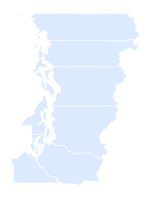
plot() draws the geometry column.
Coordinates and Spatial Joins
Coordinates Need Units
- A coordinate reference system (CRS) defines how coordinates locate points
- The source boundaries use NAD83 longitude and latitude in degrees,
EPSG:4269 - A degree of longitude spans different distances at different latitudes
- To measure local distances, transform to a projected CRS in meters
Transform, Then Measure
NAD83 / UTM zone 10N
metreEPSG:26910is NAD83 / UTM zone 10N, suitable for our western Washington sampleto_crs(...)changes the coordinate valuesset_crs(...)labels existing coordinates; it does not transform them- Choose the projection for your region (GeoPandas guide)
Select City Coordinates
Keep the five cities’ coordinates and shorten their map labels.
From Coordinates to Points
| city | lon | lat | |
|---|---|---|---|
| 43 | Bellingham | -122.470179 | 48.753442 |
| 185 | Everett | -122.193002 | 47.951130 |
| 419 | Olympia | -122.895000 | 47.040604 |
xis longitude,yis latitude- These Census Gazetteer coordinates use NAD83 (
EPSG:4269) - They are city reference points, not workers’ home or workplace locations
Which County Contains Each Point?
| city | GEOID | NAME | |
|---|---|---|---|
| 43 | Bellingham | 53073 | Whatcom |
| 185 | Everett | 53061 | Snohomish |
| 419 | Olympia | 53067 | Thurston |
| 507 | Seattle | 53033 | King |
| 560 | Tacoma | 53053 | Pierce |
The spatial join assigns a county ID from each point’s location.
Map the City Points
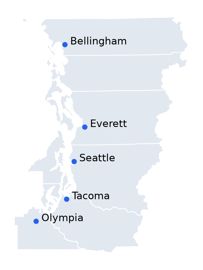
The same operation assigns establishments, schools, or transactions to areas.
Attribute and Spatial Joins
| Operation | Matching rule | Example |
|---|---|---|
merge |
Equal identifiers | County unemployment rate → county polygon |
sjoin |
A geometric relationship | Establishment coordinates → county polygon |
- Before a spatial join, put both tables in the same CRS
- A left join retains unmatched rows; inspect missing and multiple matches
withinexcludes points exactly on a boundary- Precise assignments near borders require more detailed boundaries
Commuting Tables and Maps
Load the Commuting Table
| home_state | home_county | work_state | work_county | workers | |
|---|---|---|---|---|---|
| 0 | 01 | 001 | 001 | 001 | 8671 |
| 1 | 01 | 001 | 001 | 003 | 8 |
| 2 | 01 | 001 | 001 | 007 | 11 |
- Read geographic codes as strings to preserve leading zeros
workersis an ACS estimate for workers age 16+, not a count of daily trips;moeis its 90% margin of error
Make County IDs Agree
| home_id | work_id | workers | |
|---|---|---|---|
| 0 | 01001 | 01001 | 8671 |
| 1 | 01001 | 01003 | 8 |
| 2 | 01001 | 01007 | 11 |
- A county ID joins the two-digit state code and three-digit county code
- Workplace-state codes include a country prefix; take their last two digits
- Foreign and unspecified workplaces have missing county IDs; retain these workers in home-county totals
What Does a Flow Measure?
Let \(L_{ij}\) be the reported number of workers who live in \(i\) and work in \(j\).
\[ R_i = \sum_j L_{ij}, \qquad W_i = \sum_j L_{ji} \]
- \(R_i\): workers counted by residence; \(W_i\): workers counted by workplace
- \(L_{ii}\): workers who live and work in the same county, including those working from home
- Sum all reported origins and destinations, including those outside our region
- These are pooled 2016–2020 survey estimates. An absent pair is not an observed zero
Keep Flows across the Sample Boundary
touches_region = flows.home_id.isin(county_ids)
touches_region |= flows.work_id.isin(county_ids)
flows = flows.loc[touches_region].copy()
residents = flows.groupby("home_id").workers.sum().rename("residents")
workplaces = flows.groupby("work_id").workers.sum().rename("workplaces")
same_county = flows.loc[flows.home_id == flows.work_id]
local = same_county.groupby("home_id").workers.sum().rename("local")- Keep a flow when either endpoint is in the region: 1,155 reported pairs
- County totals include commuters entering and leaving the region
Merge County Totals
| NAME | residents | workplaces | |
|---|---|---|---|
| 41 | Island | 38203 | 29416 |
| 1094 | King | 1200041 | 1403665 |
| 1208 | Kitsap | 128516 | 119863 |
Join on GEOID, keeping the county geometry.
Commuting Shares
\[ \text{out-share}_i = 1 - \frac{L_{ii}}{R_i}, \qquad \text{in-share}_i = 1 - \frac{L_{ii}}{W_i} \]
| NAME | out_share | in_share | |
|---|---|---|---|
| 41 | Island | 0.307 | 0.100 |
| 1094 | King | 0.064 | 0.200 |
| 1208 | Kitsap | 0.177 | 0.118 |
Out-share: share of resident workers working outside the county. In-share: share of workers in the county living elsewhere.
Map the Out-Commuting Share
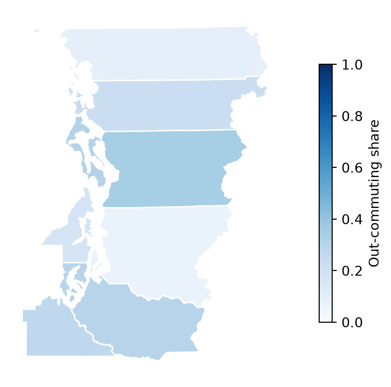
Color shows the share from 0 to 1; polygon size reflects area, not worker counts.
Why the Sample Boundary Matters
GEOID
53029    0.989
53033    0.994
53035    0.981
53053    0.989
53057    0.993
53061    0.994
53067    0.942
53073    0.984
Name: share_kept, dtype: float64
Restricting both endpoints first would remove some commuters from the denominators.
County-Pair Distances
Match Population Centers by County ID
Join the population centers to county polygons using the five-digit GEOID.
Which Center Represents a County?
- A geometric centroid weights area; a population center weights people
- Population centers approximate both endpoints; workplace locations may differ
Attach the Two Endpoints
- Each row is a directed origin–destination pair
- Omit same-county pairs: their zero center-to-center distance does not measure travel
Distances in Kilometers
| home_id | work_id | workers | distance_km | |
|---|---|---|---|---|
| 113421 | 53029 | 53033 | 2149 | 77.4 |
| 113422 | 53029 | 53035 | 69 | 66.2 |
| 113424 | 53029 | 53053 | 41 | 115.0 |
| 113426 | 53029 | 53057 | 3274 | 34.0 |
| 113427 | 53029 | 53061 | 5537 | 42.4 |
distance measures straight-line separation for each pair, not road distance or travel time.
Draw Connections to King County
Each line connects a home county’s population center to King’s.
Commuting to King County
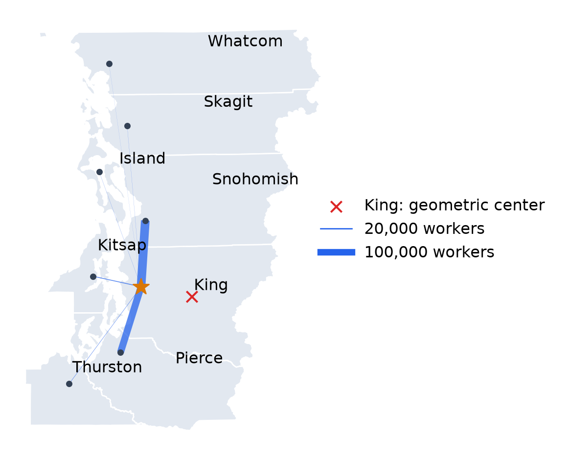
King’s geometric center (red ×) lies east of its population center (gold ★). Line widths show workers to King.
Export the County Table
| GEOID | NAME | residents | workplaces | out_share | in_share | |
|---|---|---|---|---|---|---|
| 41 | 53029 | Island | 38203 | 29416 | 0.307 | 0.100 |
| 1094 | 53033 | King | 1200041 | 1403665 | 0.064 | 0.200 |
| 1208 | 53035 | Kitsap | 128516 | 119863 | 0.177 | 0.118 |
build/spatial_county_analysis.csvhas one row per countypairshas one row per reported directed county pair
Estimating Commuting Gravity
The Paper’s Commuting Regression
- Monte et al. (2018) estimate a gravity equation in Appendix B.6, equation (B.74)
\[ \log L_{ij} = \alpha_i + \delta_j + \beta \log d_{ij} + u_{ij} \]
- \(\alpha_i\): residence fixed effect; \(\delta_j\): workplace fixed effect
- \(\beta\): distance elasticity of commuting flows
- Dividing counts by the national total, as in the paper, only changes the intercept
Pooled OLS
- The 53 pairs have positive flows and distances; each receives equal weight
- The pooled slope mixes distance with county size and attractiveness
Residence and Workplace Fixed Effects
C(...)adds county indicators, omitting reference categories- Residence effects absorb origin factors such as the number of resident workers
- Workplace effects absorb destination factors such as employment size
Compare the Estimates
| Pooled OLS | Residence + workplace FE | |
|---|---|---|
| Distance elasticity | -3.244 | -3.744 |
| R-squared | 0.519 | 0.899 |
| Pairs | 53.000 | 53.000 |
- The distance relationship is steeper after adding county effects
- \(R^2\) measures in-sample fit; the fixed-effects model also uses more parameters
Remove County Effects
- Regress each variable on the same residence and workplace effects
- Plot the residuals against each other
- Their fitted slope equals the full regression’s distance coefficient (Frisch–Waugh–Lovell)
Commuting Gravity
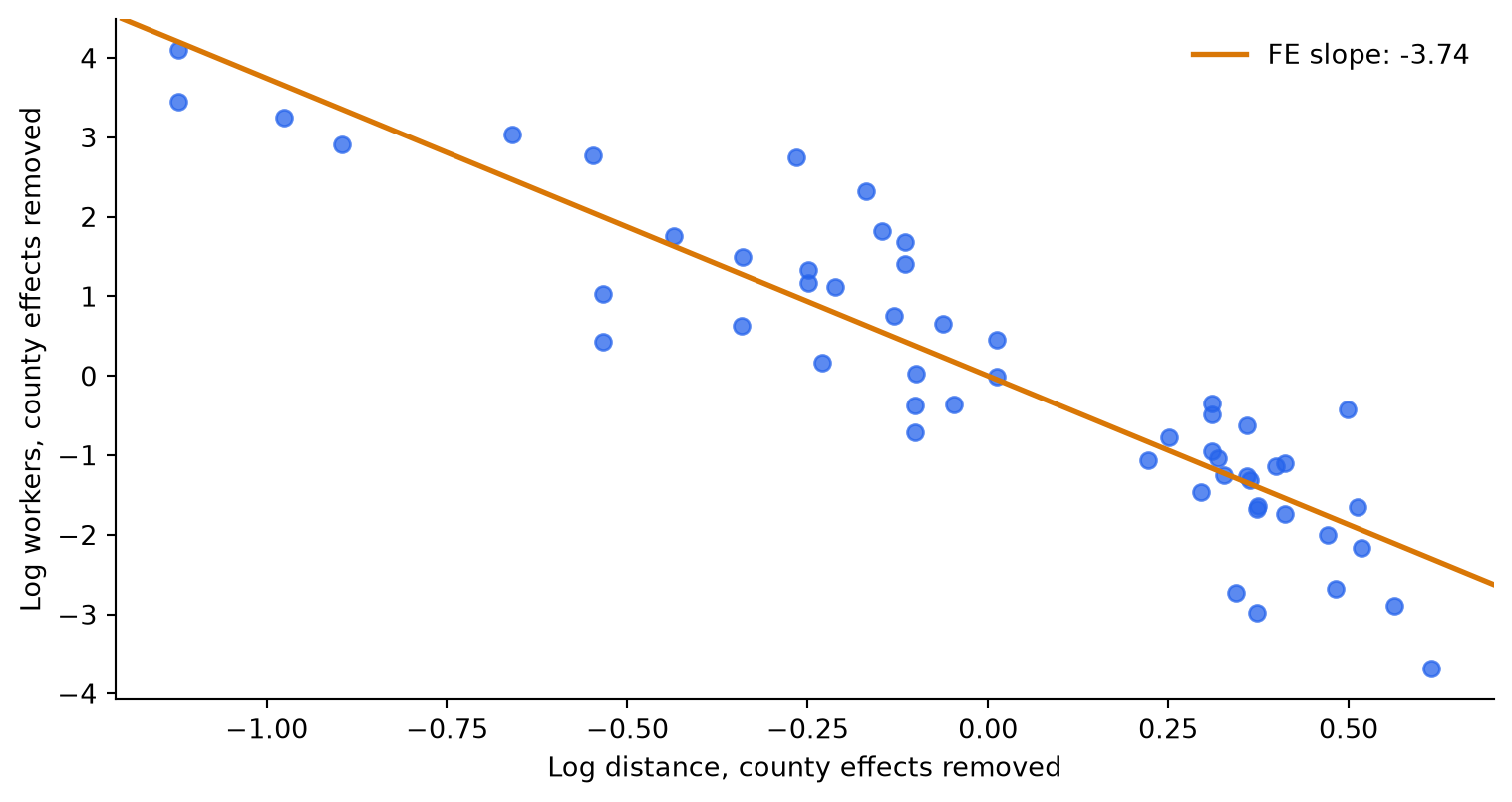
The same residual plot as Figure B.5, using our sample and population-center distances.
Interpret the Distance Elasticity
Holding county effects fixed, doubling distance multiplies the fitted flow by \(2^{\hat\beta}\).
Distance elasticity: -3.74
Fitted change when distance doubles: -92.5%- Commuting falls sharply with distance, conditional on county effects
- The paper estimates \(-4.43\) with national 2006–2010 data, centroid distances, and adjusted flows
- This association does not identify employment responses to plant openings; the paper studies those separately
References
Fleischmann, Martin, Joris Van den Bossche, Kelsey Jordahl, et al. 2026. “GeoPandas: Fundamental Data Structures for Vector Spatial Data in Python.” Computers, Environment and Urban Systems 130: 102495. https://doi.org/10.1016/j.compenvurbsys.2026.102495.
Monte, Ferdinando, Stephen J. Redding, and Esteban Rossi-Hansberg. 2018. “Commuting, Migration, and Local Employment Elasticities.” American Economic Review 108 (12): 3855–90. https://doi.org/10.1257/aer.20151507.