Probability and Uncertainty

Graduate Quantitative Economics and Datascience

Jesse Perla

jesse.perla@ubc.ca

University of British Columbia

Table of contents

• Overview
• Review: Probability SpacesOptional
• Discrete Distributions
• LLN and CLT
• Joint Distributions
• Expectations
• ReviewQuestions
• Calculating with Bivariate DistributionsOptional

Overview

Motivation

• Discrete distributions and their expectations are linear algebra: probabilities and values are vectors, expectations are dot products
• Simulating draws, and what the law of large numbers and central limit theorem say about sample means
• Joint, marginal, and conditional distributions, independence, Simpson’s paradox, and Bayes’ law
• Conditional and iterated expectations, which return throughout econometrics and machine learning
• The first section reviews the definitions of probability spaces and is optional

Extra Materials

• QuantEcon Probability
• QuantEcon Meaning of Probability
• QuantEcon Distributions and Probabilities
• QuantEcon LLN and CLT

Packages

import matplotlib.pyplot as plt
import numpy as np
import scipy.stats
import seaborn as sns
from matplotlib.animation import FuncAnimation
import IPython.display

Review: Probability SpacesOptional

Definitions

To formalize probability always be careful to separate

1. Events i.e., probability space.
2. Probability an event occurs. i.e., probability measure
3. Value or implications of an event. i.e., random variables

Probability Space

Probability space is a triple \((\Omega, {\mathcal{A}}, \mathbb{P})\):

• Set \(\Omega\) of possible outcomes and \(\omega \in \Omega\) is a particular outcome

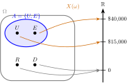
  • e.g. \(\Omega = \{U, E, R, D\}\) for unemployed, employed, retired, or dead

• Subsets \(A \subseteq \Omega\) are events

  • e.g. \(A = \{U, E\}\) is the event of being employed or unemployed
  • \(\Omega \setminus A = \{R, D\}\) (the \setminus) is event of not being either

• A probability measure \(\mathbb{P}\) assigning a probability to each event (next slides)

• The collection of all possible events is \({\mathcal{A}}\) where \(A \in {\mathcal{A}}\)

  • \(\Omega \in {\mathcal{A}}\), i.e. we can consider the event of any outcome occurring
  • \(\emptyset \in {\mathcal{A}}\), i.e. we can consider the event of nothing occurring

Probability Measure

Probability Measure is a function which assigns a numerical value on the likelihood of an event

• For us, \(\mathbb{P}: {\mathcal{A}}\rightarrow [0,1]\)

  • e.g. \(\mathbb{P}(\{U, E\}) = 0.7\) is probability either \(U\) or \(E\)
  • \(\mathbb{P}(\Omega \setminus \{U, E\}) = 0.3\)

• Will see denoted as a function, \(\mu(A)\) for integrals in advanced uses

  • Overkill for probability spaces with a finite, discrete number of elements
  • Important for probability spaces with a continuous number of elements
  • Essential for stochastic processes (e.g., flipping a coin until heads)

Random Variables

Random Variable: \(X(\omega)\) assigns a numerical value to a particular outcome

• \(X : \Omega \rightarrow {\mathbb{R}}\), but could be vector or matrix valued

  • e.g. \(X(\omega = E) = 1\) if employed, \(X(\omega = U) = 0\) if unemployed. Useful for doing counts

• Or \(X(\omega = E) = \$40,000\) if employed, \(X(\omega = U) = \$15,000\) if unemployed. Useful for finding average incomes

• Random variables defined on \(\Omega\), and inherit the probability measure

  • So can query values like \(\mathbb{P}(X =\$40,000)\)

Outcomes, Events, and a Random Variable

• The event \(A = \{U, E\}\) is a subset of \(\Omega\); the random variable \(X(\omega)\) maps each outcome to a number, and outcomes can share a value

Axioms of Probability

Probability measure \(\mathbb{P}\) on the measurable space \((\Omega, {\mathcal{A}})\) must satisfy axioms:

• Non-negativity: \(\mathbb{P}(A) \geq 0\)
• Normalization: \(\mathbb{P}(\Omega) = 1\)
• Additivity: If \(A \cap B = \emptyset\), then \(\mathbb{P}(A \cup B) = \mathbb{P}(A) + \mathbb{P}(B)\)

These imply other results such as:

• \(\mathbb{P}(\emptyset) = 0\)
• \(\mathbb{P}(A \cup B) = \mathbb{P}(A) + \mathbb{P}(B) - \mathbb{P}(A \cap B)\)
• \(\mathbb{P}(\Omega \setminus A) = 1 - \mathbb{P}(A)\)

Discrete Distributions

Discrete Distributions

• Discrete probability spaces have a finite (or countable) number of outcomes

• When convenient, we can number the outcomes arbitrarily as \(n = 1,\ldots N\) (or \(\infty\)) and then work with \(\Omega = \{1, \ldots N\}\) and \(\omega \in \Omega\)

• Axioms especially simple because we use \(\mathbb{P}(\omega = n) = p_n\),

  • Non-negativity: \(p_n \geq 0\)
  • Normalization: \(\sum\limits_{n=1}^{N} p_n = 1\)
  • Additivity: \(\mathbb{P}(A) = \sum\limits_{n \in A} p_n\)

• A random variable attaches a value \(x_n\) to each outcome. If several outcomes share a value, add their probabilities to get the probability of that value

Question What Is the Missing Probability?

\(X\) takes exactly three possible values, with probabilities

\[ 0.2,\quad 0.5,\quad p. \]

What must \(p\) be?

A. \(0.2\)
B. \(0.3\)
C. \(0.5\)
D. \(0.7\)

PMF and CDF

• For distinct values \(x_1, \ldots, x_N\), the Probability Mass Function (PMF) gives the probability of each value of \(X\)

\[ p_n \equiv \mathbb{P}(X = x_n) \]

• The Cumulative Distribution Function (CDF) gives the probability that \(X\) is at most a threshold \(t\)

\[ F(t) \equiv \mathbb{P}(X \leq t) = \sum_{n:\,x_n \leq t} p_n \]

Expectations

• The expectation of a random variable is the sum of its values weighted by their probabilities, and the same for any function \(f\) of it
• Let \(x \equiv \begin{bmatrix} x_1 & \ldots & x_N \end{bmatrix}^{\top}\) be the values and \(p \equiv \begin{bmatrix} p_1 & \ldots & p_N \end{bmatrix}^{\top}\) the probabilities, with \(f(\cdot)\) broadcast across \(x\)

\[ \begin{aligned} {\mathbb{E}}[X] &= \sum_{n=1}^N x_n \mathbb{P}(X = x_n) = p^{\top} x\\ {\mathbb{E}}[f(X)] &= \sum_{n=1}^N f(x_n) \mathbb{P}(X = x_n) = p^{\top} f(x) \end{aligned} \]

• If \(X\) has a probability density, replace the sums with integrals

Example with a Discrete Distribution

• \(\Omega = \{U, E, R\}\)
• \(\mathbb{P}(U) = 0.1, \mathbb{P}(E) = 0.8, \mathbb{P}(R) = 0.1\)
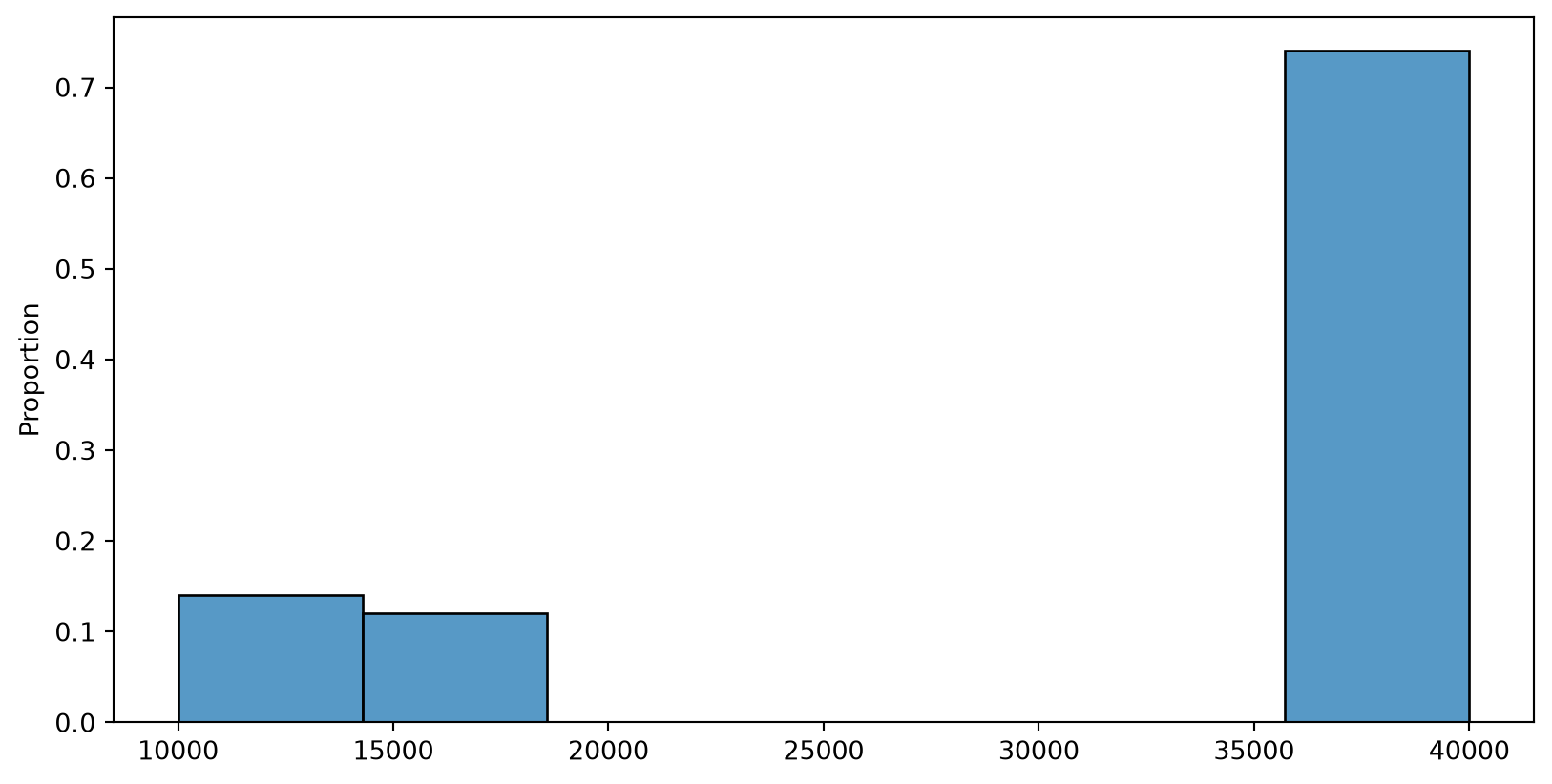
• \(X(U) = 15000, X(E) = 40000, X(R) = 10000\)
• \({\mathbb{E}}[X]\) and \({\mathbb{E}}[\sqrt{X}]\)

p = np.array([0.1, 0.8, 0.1])
x = np.array([15000, 40000, 10000])
def f(x):
    return np.sqrt(x)
print(f"E(X) = {p @ x}")
print(f"E(f(X)) = {p @ f(x)}")
order = np.argsort(x)
print(f"Sorted x = {x[order]}")
print(f"CDF(X) = {np.cumsum(p[order])}")

E(X) = 34500.0
E(f(X)) = 182.2474487139159
Sorted x = [10000 15000 40000]
CDF(X) = [0.1 0.2 1. ]

Sort the values and their probabilities together before taking cumulative sums

Using scipy.stats.rv_discrete

• rv_discrete takes distinct values and their probabilities; it sorts them internally
• Gives the mean, expectations of functions, the CDF, and random draws

p = np.array([0.1, 0.1, 0.8])
x = np.array([10000, 15000, 40000])
dist = scipy.stats.rv_discrete(
  values=(x, p))
samples = dist.rvs(size=5)
print(f"E(X) = {dist.mean()}")
print(f"E(f(X)) = {dist.expect(f)}")
print(f"CDF(X) = {dist.cdf(x)}")
print(f"Samples of X = {samples}")

E(X) = 34500.0
E(f(X)) = 182.2474487139159
CDF(X) = [0.1 0.2 1. ]
Samples of X = [40000 40000 40000 40000 15000]

Histograms of 50 and 500 Draws

fig, axes = plt.subplots(1, 2, figsize=(14, 5))
for n_draws, ax in zip([50, 500], axes):
    sns.histplot(dist.rvs(size=n_draws), stat="proportion", ax=ax)
    ax.set_title(f"{n_draws} draws")
plt.show()

Histograms of 50 and 500 Draws

The Binomial Distribution

The binomial distribution counts successes in \(N\) independent trials, each with success probability \(\theta\). For \(n = 0, \ldots, N\),

\[ \begin{aligned} \mathbb{P}(X = n) &= \binom{N}{n} \theta^n (1-\theta)^{N-n}\\ {\mathbb{E}}[X] &= \sum_{n=0}^N n \binom{N}{n} \theta^n (1-\theta)^{N-n} = N \theta \end{aligned} \]

n_trials = 10
theta = 0.5
dist = scipy.stats.binom(n_trials, theta)
print(f"Mean: {dist.mean():.2f}")
print(f"Variance: {dist.var():.2f}")
print(f"Draws: {dist.rvs(5)}")

Mean: 5.00
Variance: 2.50
Draws: [6 2 6 4 4]

The Binomial Probability Mass Function

grid = np.arange(n_trials + 1)
pmf = dist.pmf(grid)

fig, ax = plt.subplots()
ax.plot(grid, pmf,
  linestyle='',
  marker='o',
  alpha=0.8, ms=4)
ax.vlines(grid, 0,
  pmf,
  lw=0.2)
ax.set_xticks(grid)
plt.show()

The Binomial Cumulative Distribution Function

\[ \mathbb{P}(X \leq n) = \sum_{i=0}^n \binom{N}{i} \theta^i (1-\theta)^{N-i} \]

grid = np.arange(n_trials + 1)
cdf = dist.cdf(grid)

fig, ax = plt.subplots()
ax.step(grid, cdf, where="post")
ax.vlines(grid, 0, cdf,
  lw=0.2)
ax.set_xticks(grid)
plt.show()

Histograms of 50 and 5000 Binomial Draws

fig, axes = plt.subplots(1, 2, figsize=(14, 5))
for n_draws, ax in zip([50, 5000], axes):
    ax.hist(dist.rvs(size=n_draws), bins=np.arange(n_trials + 2) - 0.5,
            density=True)
    ax.set_title(f"{n_draws} draws")
plt.show()

Histograms of 50 and 5000 Binomial Draws

LLN and CLT

Law of Large Numbers (LLN)

• Take independent, identically distributed random variables \(X_1, X_2, \ldots\) with \({\mathbb{E}}|X_n| < \infty\) and \({\mathbb{E}}[X_n] = \mu\). A finite variance is not needed

• The sample mean \(\bar{X}_N \equiv \frac{1}{N}\sum_{n=1}^N X_n\) is itself a random variable

• The weak law says that for any \(\epsilon > 0\)

  \[ \lim_{N\to\infty} \mathbb{P}(|\bar{X}_N - \mu| > \epsilon) = 0 \]

  • Denoted \(\bar{X}_N \xrightarrow{p} \mu\), “convergence in probability”. The strong law strengthens this to convergence with probability one under the same assumptions

• Powerful and frequently used, but remember the assumptions!

Visualizing the LLN with Gaussian Draws

mu, sigma = 0, 1
fig, axes = plt.subplots(1, 2, figsize=(14, 5))
for n_draws, ax in zip([20, 100], axes):
    np.random.seed(42)
    samples = np.random.normal(mu, sigma, n_draws)
    t = np.arange(1, n_draws + 1)
    sample_means = np.cumsum(samples) / t
    ax.scatter(t, samples, label="Draws", alpha=0.6, s=10)
    ax.plot(t, sample_means, label="Sample mean", lw=2)
    ax.axhline(mu, color="r", linestyle="--", label="True mean")
    ax.vlines(t, sample_means, samples, color="gray", lw=0.5)
    ax.set(title=f"$N = {n_draws}$", xlabel="Draw number")
axes[0].legend()
plt.show()

Visualizing the LLN with Gaussian Draws

Pareto Distributions

• Pareto distributions are a family of distributions with a power-law tail
• For \(x_m > 0\) and \(\alpha > 0\), the PDF is

\[ p(x) = \frac{\alpha x_m^{\alpha}}{x^{\alpha+1}},\quad x \geq x_m \]

• The density is zero for \(x < x_m\)
• The mean is \({\mathbb{E}}[X] = \frac{\alpha x_m}{\alpha - 1}\) for \(\alpha > 1\)
• The variance is \(\operatorname{Var}[X] = \frac{\alpha x_m^2}{(\alpha - 1)^2(\alpha - 2)}\) for \(\alpha > 2\)
• With \(\alpha = 1.5\) the mean is finite but the variance is infinite: the LLN still holds, slowly, while the CLT below does not apply

A power-law density tail has \(p(x) \sim C x^{-\gamma}\) as \(x \to \infty\), with \(C > 0\) and \(\gamma > 1\). The Pareto has \(\gamma = \alpha + 1\)

Visualizing the Sample Means for a Pareto Distribution

n_draws = 100
np.random.seed(42)
dist = scipy.stats.pareto(1.5)
samples = dist.rvs(size=n_draws)
t = np.arange(1, n_draws + 1)
sample_means = np.cumsum(samples) / t
fig, ax = plt.subplots(figsize=(11, 5))
ax.scatter(t, samples, label="Draws", alpha=0.6, s=10)
ax.plot(t, sample_means, label="Sample mean", lw=2)
ax.axhline(dist.mean(), color="r", linestyle="--", label="True mean")
ax.vlines(t, sample_means, samples, color="gray", lw=0.5)
ax.set(xlabel="Draw number")
ax.legend()
plt.show()

Visualizing the Sample Means for a Pareto Distribution

Central Limit Theorem (CLT)

• The Central Limit Theorem (CLT) is a classic result in statistics

• Again, assume IID observations with \({\mathbb{E}}[X_n] = \mu\) and \(0 < \operatorname{Var}[X_n] = \sigma^2 < \infty\)

• Define the sample mean \(\bar{X}_N \equiv \frac{1}{N} \sum_{n=1}^N X_n\)

• Then the CLT is

  \[ \sqrt{N} \left( \bar{X}_N - \mu \right) \xrightarrow{d} {\mathcal{N}}(0, \sigma^2) \]

  • That notation means converges in distribution, which roughly means that as \(N\to\infty\) the CDFs are getting closer to each other

Visualizing the CLT with Exponential Distributions

• See QuantEcon CLT lecture for the source.
• Exponential density \(p(x) = \lambda e^{-\lambda x}\) for \(x \geq 0\), and zero otherwise; here \(\lambda = 0.5\)

dist = scipy.stats.expon(scale=1/0.5)
mu, s = dist.mean(), dist.std()
x = np.linspace(0, 15.0, 1000)
y = dist.pdf(x)
plt.plot(x, y)
plt.xlabel('Value')
plt.ylabel('Density')
plt.show()

CLT for Exponential Draws

fig, ax = plt.subplots()
def update(n):
    ax.clear()
    data = dist.rvs((10000, n))
    Y = np.sqrt(n) * (data.mean(axis=1) - mu)
    ax.set_xlim(-3 * s, 3 * s)
    ax.set_ylim(0, 0.5)
    ax.hist(Y, bins=60, alpha=0.5, density=True)
    ax.set_title(f"CLT for $N = {n}$")
    x = np.linspace(-3 * s, 3 * s, 100)
    pdf = scipy.stats.norm.pdf(x, 0, s)
    ax.plot(x, pdf, "r-", lw=2, label=r"$\mathcal{N}(0, \sigma^2)$")
    ax.legend()
frames = [1, 2, 3, 5, 10, 20, 50, 100, 500, 2000]
ani = FuncAnimation(fig, update, frames=frames, interval=500, repeat=False)
plt.close()
IPython.display.HTML(ani.to_html5_video())

CLT for Exponential Draws

Question LLN, CLT, or Both?

The observations are IID Pareto draws with \(\alpha = 1.5\).

The mean is finite, but the variance is infinite.

Which result applies to their sample mean?

A. Both the LLN and the usual finite-variance CLT
B. The usual CLT, but not the LLN
C. The LLN, but not the usual finite-variance CLT
D. Neither result

Joint Distributions

Joint Probability Distributions

• Key concepts are marginal distributions, conditional distributions, independence, and conditional expectations
• Will demonstrate with bivariate discretely valued distributions
  • Similar for multivariate distributions, except we replace sums with sums over multiple indices
  • Similar for continuous or mixed discrete-continuous distributions, except we replace sums with integrals
• Interpretation of the joint distribution of \(X\) and \(Y\) is the probability of each pair of outcomes occurs
  • e.g., prob you get a cash transfer and are unemployed, don’t get a cash transfer and are unemployed, get a cash transfer and are employed, etc.

Bivariate Probability Distributions

• Let \(X,Y\) be two discrete random variables that take values:

  \[ X\in\{1,\ldots,I\},\quad Y\in\{1,\ldots,J\} \]

• Then their joint distribution is described by a matrix

  \[ P\equiv[\mathbb{P}(X=i,Y=j)]_{i=1\ldots I, j=1,\ldots J}\in {\mathbb{R}}^{I\times J} \]

• Which fulfills the key axioms of probability

\[ \begin{aligned} p_{ij}\equiv\mathbb{P}(X=i,Y=j) &\geq 0\\ \sum_{i=1}^{I}\sum_{j=1}^{J}p_{ij}=1 \end{aligned} \]

Marginal Probability Distributions

• The joint distribution induces marginal distributions

  \[ \begin{aligned} \mathbb{P}(X=i)& = \sum_{j=1}^{J}p_{ij} = \mu_i, \quad i=1,\ldots,I\\ \mathbb{P}(Y=j)&= \sum_{i=1}^{I}p_{ij} = \nu_j, \quad j=1,\ldots,J \end{aligned} \]

• The marginal distributions are also probability distributions

  • i.e., \(\mu_i \geq 0\) and \(\sum_{i=1}^{I} \mu_i = 1\)
  • e.g. the probability you were given a conditional cash transfer regardless of your employment status

Calculating Marginal Distributions

• Take a bivariate \(\mathbb{P}(X=i, Y=j)\) with \(I=5\) and \(J=4\)
• Row sums of \(P\) give \(\mathbb{P}(X=i) = \mu_i\) and column sums give \(\mathbb{P}(Y=j) = \nu_j\); the numpy version is in the optional section

\[ P = \begin{bmatrix} 0.05 & 0.07 & 0.02 & 0.01 \\ 0.04 & 0.10 & 0.06 & 0.03 \\ 0.08 & 0.09 & 0.07 & 0.04 \\ 0.02 & 0.03 & 0.02 & 0.01 \\ 0.09 & 0.08 & 0.04 & 0.05 \end{bmatrix},\quad \mu = \begin{bmatrix} 0.15 \\ 0.23 \\ 0.28 \\ 0.08 \\ 0.26 \end{bmatrix},\quad \nu = \begin{bmatrix} 0.28 & 0.37 & 0.21 & 0.14 \end{bmatrix} \]

• \(P\), \(\mu\), and \(\nu\) each sum to \(1\)

Conditional Probability

• For \(\mathbb{P}(B) > 0\), conditional probabilities are defined by

  \[ \mathbb{P}(A \,|\, B)=\frac{\mathbb{P}(A \cap B)}{\mathbb{P}(B)} \]

• \(A \cap B\) is the event that both \(A\) and \(B\) occur, i.e., the intersection

  • e.g. you were given a conditional cash transfer AND you were unemployed

• The conditional probability is the probability of \(A\) given \(B\) has occurred

  • e.g. the probability you were given a conditional cash transfer given you were unemployed

Conditional Distributions

For discrete random variables with \(\mathbb{P}(Y=j) > 0\), the conditional distribution is

\[ \mathbb{P}(X=i|Y=j)=\frac{p_{ij}}{\sum_{k=1}^{I}p_{kj}} =\frac{\mathbb{P}(X=i, Y=j)}{\mathbb{P}(Y=j)} \]

• Fix \(Y=j\). The probabilities are nonnegative since \(p_{ij} \geq 0\), and they sum to \(1\)

\[ \sum_{i=1}^{I}\mathbb{P}(X=i\,|\,Y=j) =\frac{\sum_{i=1}^{I}p_{ij}}{\sum_{k=1}^{I}p_{kj}}=1 \]

Question Condition on Which Group?

This table gives \(\mathbb{P}(X=i, Y=j)\).

	\(Y=1\)	\(Y=2\)
\(X=1\)	0.10	0.20
\(X=2\)	0.30	0.40

What is \(\mathbb{P}(X=1\,|\,Y=1)\)?

A. \(0.10\)
B. \(0.25\)
C. \(0.30\)
D. \(0.40\)

Law of Total Probability

• Law of Total Probability is a useful identity for conditional probabilities

  • Let \(A_1, \ldots, A_N\) partition \(\Omega\), with \(\mathbb{P}(A_i) > 0\)
  • i.e., \(\Omega = \cup_{i=1}^{N} A_i\) and \(A_i \cap A_j = \emptyset\) for \(i \neq j\)

• Then for any event \(B\),

  \[ \mathbb{P}(B) = \sum_{i=1}^{N} \mathbb{P}(B \cap A_i) = \sum_{i=1}^{N} \mathbb{P}(B \,|\, A_i) \mathbb{P}(A_i) \]

  • e.g. the probability of being unemployed is the probability of being unemployed and getting a cash transfer plus the probability of being unemployed and not getting a cash transfer

Statistical Independence

• Random variables \(X\) and \(Y\) with marginals \(\mu\) and \(\nu\) are statistically independent if

  \[ \mathbb{P}(X=i,Y=j)=\mu_i \nu_j,\text{ for all } i, j \]

  • i.e., the joint distribution is the product of the marginal distributions
  • e.g., the probability you were given a conditional cash transfer AND you were unemployed is probability you were given a conditional cash transfer \(\times\) the probability you were unemployed

Conditional Distributions and Independence

• When \(X\) and \(Y\) are independent and \(\nu_j = \mathbb{P}(Y=j) > 0\),

  \[ \begin{aligned} \mathbb{P}(X=i\,|\,Y=j) &=\frac{\mathbb{P}(X=i, Y=j)}{\mathbb{P}(Y=j)} =\frac{\mu_i \nu_j}{\sum_{k=1}^{I}\mu_k \nu_j} =\frac{\mu_i \nu_j}{\nu_j\sum_{k=1}^{I}\mu_k}=\frac{\mu_i \nu_j}{\nu_j\times 1}=\mu_i \\ \end{aligned} \]

• Thus independence implies the conditional distributions are the marginals:

  • \(\mathbb{P}(X=i\,|\,Y=j) = \mathbb{P}(X=i)\)
  • Similarly, \(\mathbb{P}(Y=j\,|\,X=i) = \mathbb{P}(Y=j)\)

Notation for (Conditional) Independence

• Let \(X, Y, Z\) be discrete random variables; condition only on values with positive probability

• Common notation for independence is

  \[ \begin{aligned} X &\perp\!\!\!\perp Y\\ \mathbb{P}(X=x, Y=y) &= \mathbb{P}(X=x) \mathbb{P}(Y=y) \end{aligned} \]

• Common notation for conditional independence

  \[ \begin{aligned} X &\perp\!\!\!\perp Y \,|\, Z\\ \mathbb{P}(X=x, Y=y\,|\, Z=z) &= \mathbb{P}(X=x\,|\, Z=z) \mathbb{P}(Y=y\,|\, Z=z) \end{aligned} \]

• Central to causal inference and treatment effects

Classic Example of Conditional Independence

• Let \(X\) be a child’s shoe size
• Let \(Y\) be the child’s reading ability
• Let \(Z\) be the child’s age
• Across children, both can grow with age. Suppose that within each age group, shoe size tells us nothing about reading ability
  • Then \(X \perp\!\!\!\perp Y \,|\, Z\): conditional independence is a modeling assumption here, not something implied by both growing with age

Simpson’s “Paradox”

• Simpson’s paradox is a warning on composition effects

• Let \(S\) be the event of admission, \(G\) gender, and \(D\) department. By the law of total probability

  \[ \mathbb{P}(S \,|\, G) = \sum_{d} \mathbb{P}(S \,|\, G, D=d)\, \mathbb{P}(D=d \,|\, G) \]

  • A group’s overall admission rate is its department rates weighted by where the group applies

• So \(\mathbb{P}(S \,|\, G=\text{men}) > \mathbb{P}(S \,|\, G=\text{women})\) is consistent with \(\mathbb{P}(S \,|\, G=\text{men}, D=d) \leq \mathbb{P}(S \,|\, G=\text{women}, D=d)\) for every department \(d\), if women apply to departments with low admission rates

UC Berkeley Gender Bias: Overall Data

Total Applicants	Admitted	Men Applicants	Men Admitted	Women Applicants	Women Admitted
12,763	41%	8,442	44%	4,321	35%

• The Berkeley admissions study uses data from 1973
• At the unadjusted 5% threshold, 4 of the 85 departments favored men and 6 favored women; the comparison does not reverse in every department
• The biggest difference was in which departments women applied to
• The six largest departments give a sense of the heterogeneity

Conditional Probabilities for 6 Largest Departments

Dept	All Applicants	Admitted	Men Applicants	Men Admitted	Women Applicants	Women Admitted
A	933	64%	825	62%	108	82%
B	585	63%	560	63%	25	68%
C	918	35%	325	37%	593	34%
D	792	34%	417	33%	375	35%
E	584	25%	191	28%	393	24%
F	714	6%	373	6%	341	7%

Yellow: the gender with more applicants to the department. Green: the admission rate of the gender with fewer applicants, higher in every department.

Bold: the two departments each gender applied to most.

Explanation Using Conditional Probabilities

Overall, \(\mathbb{P}(\text{Admitted} \,|\, \text{Men}) = 0.44\) and \(\mathbb{P}(\text{Admitted} \,|\, \text{Women}) = 0.35\)

But this is different when conditioning on departments!

• \(\mathbb{P}(\text{Admitted} \,|\, \text{Men, Dept A}) = 0.62\), \(\mathbb{P}(\text{Admitted} \,|\, \text{Women, Dept A}) = 0.82\)
• \(\mathbb{P}(\text{Admitted} \,|\, \text{Men, Dept B}) = 0.63\), \(\mathbb{P}(\text{Admitted} \,|\, \text{Women, Dept B}) = 0.68\)
• The weights differ: 1,385 men applied to A and B, which admit 63-64% of applicants, while 986 women applied to C and E, which admit 25-35%
• “Paradox” because women tend to apply to more competitive departments

Does this Old Data Imply There was No Bias?

• All data requires assumptions to interpret! Most assumptions are implicit, so you need to reflect on what assumptions you may have made
• This simply corrected for the mechanical composition effect
• Interpreting bias better requires reflecting on your “model” and assumptions
  • Is average quality identical conditional on department and gender? Especially in 1973 when there was enormous selection bias?
  • What if bias leads women to apply to the more competitive departments?

Question Can the Overall Ranking Reverse?

Two groups apply to the same two departments.

Group A has a higher admission rate than group B within each department.

Must group A have the higher overall admission rate?

A. Yes: higher in every department means higher overall
B. No: the groups can apply to different departments in different proportions
C. No: group B must have the higher overall rate
D. The overall rates must be equal

Bayes Law

For \(\mathbb{P}(A) > 0\) and \(\mathbb{P}(B) > 0\), Bayes’ Law gives

\[ \mathbb{P}(A \,|\, B)=\frac{\mathbb{P}(B \,|\, A)\mathbb{P}(A)}{\mathbb{P}(B)} \]

Sometimes:

• \(\mathbb{P}(B\,|\,A)\) is called the “likelihood”
• \(\mathbb{P}(A)\) is called the “prior”
• \(\mathbb{P}(A\,|\,B)\) is called the “posterior”
• \(\mathbb{P}(B)\) is called the “marginal likelihood”, which normalizes the expression

Example with Bayes’ Law

\(A\) is the event of being unemployed, \(B\) is the event of getting a cash transfer

• \(\mathbb{P}(B\,|\,A)\) is the probability of being given a cash transfer given you were unemployed
• \(\mathbb{P}(A)\) is the probability of being unemployed within the whole distribution
• \(\mathbb{P}(A\,|\,B)\) is the probability of being unemployed given you were given a cash transfer
• \(\mathbb{P}(B)\) is the probability of being given a cash transfer within the whole distribution
• Bayes’ law: probability of being unemployed given you were given a cash transfer \(\propto\) probability of being given cash transfer given you were unemployed \(\times\) probability of being unemployed

Bayes’ Law: Cash Transfers

Let \(U\) mean unemployed and \(T\) mean receiving a cash transfer. Suppose

\(\mathbb{P}(U)=0.20\), \(\mathbb{P}(T\,|\,U)=0.80\), and \(\mathbb{P}(T\,|\,U^c)=0.20\).

1. Find the total probability of receiving a transfer:

\[ \begin{aligned} \mathbb{P}(T) &= \mathbb{P}(T\,|\,U)\mathbb{P}(U) + \mathbb{P}(T\,|\,U^c)\mathbb{P}(U^c) \\ &= 0.80(0.20) + 0.20(0.80) = 0.32. \end{aligned} \]

2. Apply Bayes’ law to find the unemployed share among recipients:

\[ \mathbb{P}(U\,|\,T) = \frac{\mathbb{P}(T\,|\,U)\mathbb{P}(U)}{\mathbb{P}(T)} = \frac{0.80(0.20)}{0.32} = 0.50. \]

So 50% of transfer recipients are unemployed.

Bayes Law with Bivariate Random Variables

• For discrete random variables with \(\mathbb{P}(X=i) > 0\) and \(\mathbb{P}(Y=j) > 0\), Bayes’ Law gives

  \[ \mathbb{P}(X=i\,|\,Y=j)=\frac{\mathbb{P}(X=i,Y=j)}{\mathbb{P}(Y=j)}=\frac{\mathbb{P}(Y=j\,|\,X=i)\mathbb{P}(X=i)}{\mathbb{P}(Y=j)} \]

• If \(X\) and \(Y\) are independent

  • \(\mathbb{P}(Y=j\,|\,X=i) = \mathbb{P}(Y=j)\)
  • Bayes’ Law simplifies to just the marginal distribution

  \[ \mathbb{P}(X=i\,|\,Y=j) = \mathbb{P}(X=i) \]

Expectations

Conditional Expectations

• For each \(j\) with \(\mathbb{P}(Y=j) > 0\), the mapping \(i \mapsto \mathbb{P}(X=i\,|\,Y=j)\) is a probability distribution over \(i\).
• A conditional expectation is an expectation using the conditional probability distribution. For a discrete random variable \(X\) and \(Y\),

\[ {\mathbb{E}}[X\,|\,Y=j] = \sum_{i=1}^{I} i\, \mathbb{P}(X=i\,|\,Y=j) \]

• If \(X\) and \(Y\) are independent then

  • Recall that \(\mathbb{P}(X=i\,|\,Y=j) = \mathbb{P}(X=i)\)
  • Which implies \({\mathbb{E}}[X\,|\,Y=j] = {\mathbb{E}}[X]\)
  • That the expected value of \(X\) is the same regardless of the value of \(Y\)

Key Properties of Expectations

• Let \(A, B\) be constants and \(X, Y\) random variables, with compatible dimensions and finite expectations for the expressions below

• Expectations are linear operators, which gives us some useful properties

  • \({\mathbb{E}}[A X + B Y] = A {\mathbb{E}}[X] + B {\mathbb{E}}[Y]\)

• \({\mathbb{E}}[X Y] \neq {\mathbb{E}}[X] {\mathbb{E}}[Y]\) in general

  • But if \(X\) and \(Y\) are independent, then \({\mathbb{E}}[X Y] = {\mathbb{E}}[X] {\mathbb{E}}[Y]\)

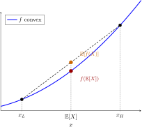
• \({\mathbb{E}}[f(X)] = f({\mathbb{E}}[X])\) is not guaranteed for nonlinear \(f\)

  • Equality always holds for affine \(f(x)=Ax+b\) or constant \(X\)

• Jensen’s Inequality: If \(f(\cdot)\) is a convex function, then \({\mathbb{E}}[f(X)] \geq f({\mathbb{E}}[X])\)

Question Square Before or After Averaging?

\(X\) equals \(0\) or \(2\), each with probability \(1/2\).

What are \({\mathbb{E}}[X]\) and \({\mathbb{E}}[X^2]\)?

A. \({\mathbb{E}}[X]=1\), \({\mathbb{E}}[X^2]=1\)
B. \({\mathbb{E}}[X]=1\), \({\mathbb{E}}[X^2]=2\)
C. \({\mathbb{E}}[X]=2\), \({\mathbb{E}}[X^2]=2\)
D. \({\mathbb{E}}[X]=2\), \({\mathbb{E}}[X^2]=4\)

Law of Total Expectations

• Let \(\{A_1, \ldots, A_N\}\) partition \(\Omega\), with \(\mathbb{P}(A_i) > 0\) and \({\mathbb{E}}|X| < \infty\)

• Law of Total Expectations

  \[ {\mathbb{E}}[X] = \sum_{i=1}^{N} {\mathbb{E}}[X \,|\, A_i] \mathbb{P}(A_i) \]

  • e.g. the expected value of income is the expected value of income given you were unemployed times the probability of being unemployed plus the expected value of income given you were employed times the probability of being employed

Related decomposition is the Law of Total Variance: \(\operatorname{Var}[X] = {\mathbb{E}}\big[\operatorname{Var}[X \,|\, Y]\big] + \operatorname{Var}\big[{\mathbb{E}}[X \,|\, Y]\big]\)

Conditional Expectations and Iterated Expectations

• Same properties all hold e.g. \({\mathbb{E}}[A X + B Y \,|\, Z] = A {\mathbb{E}}[X \,|\, Z] + B {\mathbb{E}}[Y \,|\, Z]\)

• \({\mathbb{E}}[X \,|\, Y]\) is a function of \(Y\), so it is itself a random variable

• Law of Iterated Expectations

  \[ {\mathbb{E}}\left[{\mathbb{E}}[X\,|\,Y]\right] = {\mathbb{E}}[X] \]

  • The expected value of \(X\) is the average of the conditional expectations of \(X\) given \(Y\) over the distribution of \(Y\)
  • Similarly for conditionals: \({\mathbb{E}}\left[{\mathbb{E}}[X\,|\,Y, Z]\, |\, Z\right] = {\mathbb{E}}[X\,|\,Z]\)

ReviewQuestions

Question Read the Income CDF

Income \(X\) has this distribution:

Income	Probability
\(\$10{,}000\)	\(0.10\)
\(\$15{,}000\)	\(0.10\)
\(\$40{,}000\)	\(0.80\)

What is \(\mathbb{P}(X \leq \$15{,}000)\)?

A. \(0.10\)
B. \(0.20\)
C. \(0.80\)
D. \(0.90\)

Question Are These Variables Independent?

This table gives \(\mathbb{P}(X=i, Y=j)\).

	\(Y=1\)	\(Y=2\)
\(X=1\)	0.10	0.40
\(X=2\)	0.10	0.40

Are \(X\) and \(Y\) independent?

A. Yes: every joint probability equals the product of its marginals
B. No: \(X\) and \(Y\) have different marginal distributions
C. No: the four joint probabilities are not equal
D. We cannot tell from a joint table

Question Average the Group Means

Monthly income \(X\) is in thousands of dollars.

Group	Population share	Mean income
Unemployed	\(0.25\)	\(1\)
Employed	\(0.75\)	\(3\)

What is \({\mathbb{E}}[X]\)?

A. \(2\)
B. \(2.5\)
C. \(3\)
D. \(4\)

Calculating with Bivariate DistributionsOptional

Recall: Calculating Marginal Distributions

• Lets create a bivariate \(\mathbb{P}(X=i, Y=j)\) with \(I=5\) and \(J=4\)
• Use matrix \(P\) to calculate \(\mathbb{P}(X=i)\) and \(\mathbb{P}(Y=j)\)

np.set_printoptions(precision=3)
P = np.array([[0.05, 0.07, 0.02, 0.01],
              [0.04, 0.1,  0.06, 0.03],
              [0.08, 0.09, 0.07, 0.04],
              [0.02, 0.03, 0.02, 0.01],
              [0.09, 0.08, 0.04, 0.05]])
I, J = P.shape
print(f"I = {I}, J = {J}")
print(f"sum = 1? {np.isclose(P.sum(), 1.0)}")
print(f"p_ij >= 0? {np.all(P >= 0)}")
margin_x = P.sum(axis=1) # sum over j
margin_y = P.sum(axis=0) # sum over i
print(f"P(X=i) = {margin_x}")
print(f"Sum_i P(X=i) = {margin_x.sum()}")
print(f"P(Y=j) = {margin_y}")
print(f"Sum_j P(Y=j) = {margin_y.sum()}")

I = 5, J = 4
sum = 1? True
p_ij >= 0? True
P(X=i) = [0.15 0.23 0.28 0.08 0.26]
Sum_i P(X=i) = 0.9999999999999999
P(Y=j) = [0.28 0.37 0.21 0.14]
Sum_j P(Y=j) = 1.0

Calculating Conditional Distributions

• Now use \(P\) to calculate \(\mathbb{P}(X=i\,|\,Y=j)\)

# cond_x_y[j, i] = P(X=i | Y=j);
cond_x_y = (P / margin_y).T # shape (J, I)

# cond_y_x[i, j] = P(Y=j | X=i)
cond_y_x = (P.T / margin_x).T # shape (I, J)

print(f"P(X=·|Y=1)=\n{cond_x_y[0, :]}")
print(f"P(X=·|Y=2)=\n{cond_x_y[1, :]}")
print(f"sum_i P(X=i|Y=2)={cond_x_y[1, :].sum():.2f}")
print(f"P(Y=·|X=1)=\n{cond_y_x[0, :]}")
print(f"sum_j P(Y=j|X=1)={cond_y_x[0, :].sum():.2f}")

P(X=·|Y=1)=
[0.179 0.143 0.286 0.071 0.321]
P(X=·|Y=2)=
[0.189 0.27  0.243 0.081 0.216]
sum_i P(X=i|Y=2)=1.00
P(Y=·|X=1)=
[0.333 0.467 0.133 0.067]
sum_j P(Y=j|X=1)=1.00

Calculating Conditional Expectations

• Assign an RV to each state then find \({\mathbb{E}}[X\,|\,Y=1]\)

margin_x = P.sum(axis=1)
margin_y = P.sum(axis=0)
cond_x_y = (P / margin_y).T
cond_y_x = (P.T / margin_x).T

# Give RV values to states
vals_x = np.arange(I) + 1
vals_y = np.arange(J) + 1
y_cond = 0 # Y = 1
E_x_y1 = cond_x_y[y_cond, :] @ vals_x
# non-broadcasted version
# E_x_y1 = sum(vals_x[i] * cond_x_y[y_cond, i]
#               for i in range(I))
print(f"E(X | Y = {y_cond+1})={E_x_y1}")

E(X | Y = 1)=3.214285714285715

Conditional Expectations and the Law of Iterated Expectations

# Vectorized version of E[X|Y=j] for all j
E_x_y = (cond_x_y * vals_x).sum(axis=1)  # shape (J,)
E_y_x = (cond_y_x * vals_y).sum(axis=1)  # shape (I,)

# Law of Iterated Expectations:
# E_X should equal sum_j E[X|Y=j] P(Y=j)
E_X_direct = vals_x @ margin_x
E_X_iter = E_x_y @ margin_y  # sum over j

print("E(X | Y = j) =", E_x_y)
print("E(Y | X = i) =", E_y_x)
print(f"E(X) = {E_X_direct:.3g}")
print(f"E(E(X|Y)) = {E_X_iter:.3g}")

E(X | Y = j) = [3.214 2.865 3.    3.429]
E(Y | X = i) = [1.933 2.348 2.25  2.25  2.192]
E(X) = 3.07
E(E(X|Y)) = 3.07

Check Bayes’ Law

\[ \mathbb{P}(X=1\,|\,Y=2) = \frac{\mathbb{P}(Y=2\,|\,X=1)\mathbb{P}(X=1)}{\mathbb{P}(Y=2)} \]

x = 1
y = 2
p_y_x = cond_y_x[x-1, y-1]
p_x = margin_x[x-1]
p_y = margin_y[y-1]
p_x_y = cond_x_y[y-1, x-1]
p_bayes = p_y_x * p_x / p_y
print(f"P(Y={y}|X={x}) = {p_y_x:.2g}")
print(f"P(X={x}) = {p_x:.2g}")
print(f"P(Y={y}) = {p_y:.2g}")
print(f"P(X={x}|Y={y})={p_x_y:.2g}")
print(f"P(Y={y}|X={x})P(X={x})\
/P(Y={y})={p_bayes:.2g}")

P(Y=2|X=1) = 0.47
P(X=1) = 0.15
P(Y=2) = 0.37
P(X=1|Y=2)=0.19
P(Y=2|X=1)P(X=1)/P(Y=2)=0.19

Tips for using Numpy Broadcasting

1. Don’t
   • Loops, list comprehensions (e.g., [x[i, i+1] for i in range(5)]), or a combination are usually clearer and often fast enough
2. Write the slow version first
3. Ask Github Copilot or ChatGPT to do a numpy broadcasting version
4. Test it for a few values! Easy to make mistakes
5. For more advanced usage you may be working in a ML library. If so, then packages such as jax.vmap or torch.vmap help