Natural Language Processing and Large Language Models

Graduate Quantitative Economics and Datascience

Jesse Perla

jesse.perla@ubc.ca

University of British Columbia

Overview

Summary

Discuss text, NLP, and other embeddings
Relate embeddings to transformations like PCA
Use LLMs via the LangChain package

References

These notes are a bare-bones introduction. See references for more
See Melissa Dell’s Survey Deep Learning for Economists and Course
- Topic and Sentiment Classification
- Semantic and Syntactic Similarity

API Options for LLMs

There are many ways to access these tools, including vendor-specific APIs and those which wrap things in as much of a cross-vendor way as possible
A big variation is between LLMs that are hosted and ones that run locally.
Local use of LLM/NLP is often facilitated by the package Hugging Face Transformers
- We will not use this approach here because it requires far more background, but if you are serious this is useful to know about
Remote use of LLMs can be done with
- Vendor specific APIs: e.g., OpenAI
- Cross-vendor packages: e.g., LangChain which calls out to OpenAI/Gemini/etc.

Packages

For this introduction, we will use LangChain to call out to OpenAI

from sklearn.manifold import TSNE
import matplotlib.pyplot as plt
import numpy as np
import tiktoken
from langchain_openai import ChatOpenAI, OpenAIEmbeddings
from langchain_core.messages import SystemMessage, HumanMessage, AIMessage

OpenAI via LangChain

Sign up for the OpenAI Platform
- Sometimes it is free for a limited number of tokens. See pricing for more
Go to the API keys tab and create a key
In your terminal, set OPENAI_API_KEY to this value (see here)

Creating the LangChain API

Instantiate models once (LangChain will pick up OPENAI_API_KEY from environment variable)
The model= might be chosen for speed, cost, etc.
Temperature is how random to make the output (0 = deterministic). Will discuss more later.

openai_embedding_model = "text-embedding-3-large"
openai_chat_model = "gpt-4o-mini"
llm = ChatOpenAI(model=openai_chat_model, temperature=0.7)
embedder = OpenAIEmbeddings(model=openai_embedding_model)

Tokens, Vocabulary, and Corpus

Tokens and Vocabulary

We can define a vocabulary of \(K\) possible “tokens” enumerated \(k = 1, \ldots, K\)
- For NLP, this might be common words, parts of words, and characters.
- The vocabulary is model and sometimes application specific
A splitter will take an input and break it into pieces
- e.g., take a sentence and split on the whitespace
A tokenizer will take an input and map it into a sequence of token indices
- e.g., take a sentence, split on the spaces, and then map to tokens in the vocabulary
The corpus is the set of text/etc. you use
- In specialized cases you might want to build a custom vocabulary based on how common certain words are in your corpus

Example with OpenAI Tokens

When using LLMs this sometimes happens in the background, but other times you may need more manual control
We can use a package to reverse-engineer what OpenAI does under the hood.
- Splits on whitespace, tokens may be whole words, subwords, or characters

enc = tiktoken.encoding_for_model(openai_embedding_model)
print(f"Tokens in vocabulary for {openai_embedding_model}: {enc.n_vocab}")
print(f"'Hello world' -> {enc.encode('Hello world')}")
print(f"'hello world' -> {enc.encode('hello world')}")
print(f"'hello world 67' -> {enc.encode('hello world 67')}")

Tokens in vocabulary for text-embedding-3-large: 100277
'Hello world' -> [9906, 1917]
'hello world' -> [15339, 1917]
'hello world 67' -> [15339, 1917, 220, 3080]

Tasks with Tokens

Most tasks in NLP involve working with these tokenized inputs. For example,
- Simple counts of tokens (e.g., bag of words) for comparison
- Using a sequence of tokens as input to a model to predict the next token (or missing tokens)
- Mapping a sequence of tokens into an embedding of the entire sequence for similarity/classification/etc.
Not specific to text though. Can use with any sequence of discrete or discretized outcomes

Embedding a Token

The ordering of the tokens from \(k = 1, \ldots, K\) is arbitrary
However, we can assign a real-valued vector to each token
- This is called an embedding of the token and could capture things like conceptual similarity between them, etc.
- The real-valued vectors can then be clustered, classified, etc.

Embeddings

What is an Embedding?

resp = llm.invoke([
    SystemMessage(content="You provide 2 short bullet points, technical answers."),
    HumanMessage(content="What is an embedding?")
])
resp_text = resp.content
print(resp_text)

- An embedding is a numerical representation of objects (like words, sentences, or images) in a continuous vector space, capturing semantic relationships and structures within the data.
- Commonly used in machine learning and natural language processing, embeddings facilitate tasks such as similarity measurement and clustering by allowing high-dimensional data to be represented in lower-dimensional spaces.

Detour into OpenAI (via LangChain)

Our code uses LangChain message objects to call OpenAI under the hood.
Message roles in LangChain and their OpenAI mapping:
- SystemMessage → OpenAI “system” role (sets behavior/instructions)
- HumanMessage → OpenAI “user” role (your prompt/query)
- AIMessage → OpenAI “assistant” role (model responses)
When building a conversation, you pass the entire message history (system + user + assistant) to the model each time; the model conditions on this full context.

LLMs are Stateless

When you call llm.invoke([...]) and related APIs you pass the entire history of the conversation each time.
This lets the model condition on the entire history to have history-contingent answers, and means it does not keep around a “state” or “memory” of the conversation.

Followup: What does it have to do with Latent Spaces?

resp = llm.invoke([
    SystemMessage(content="You provide 2 short bullet points, technical answers."),
    HumanMessage(content="What is an embedding?"),
    AIMessage(content=resp_text),
    HumanMessage(content="What is the relationship to latent spaces?")
])
print(resp.content)

- Latent spaces are typically the underlying representations learned by models, where embeddings serve as specific instances of points within these spaces that capture intrinsic features of the data.
- Both concepts aim to represent complex data in a more manageable form; embeddings can be viewed as mappings of data into a latent space where relationships and patterns can be more easily analyzed.

Embeddings Overview

Used loosely and inconsistently, but the spirit is the same
A mapping of some \(x \in {\mathcal{X}}\) to a latent space \(\phi(x) \in {\mathcal{Z}}\)
Typically we want that \({\mathcal{Z}}\) is a continuous vector space of finite dimension
- Crucially, we can think of distances in that space (e.g., \(||\phi(x) - \phi(y)||\))
The dimension of \({\mathcal{Z}}\) may be smaller or larger than \({\mathcal{X}}\)
- If larger, typically in only small regions of the higher-dimensional space.
Often want to preserve norms in cases where the original space itself had a norm
- e.g., if \(||x - y||\) is small, then \(||\phi(x) - \phi(y)||\) is small

Cosine Similarity

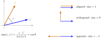
Cosine similarity is the “angle” between two vectors in the embedding space \(z = \phi(x)\) and \(z' = \phi(x')\) \[ \mathrm{sim}(z, z') = \frac{z \cdot z'}{||z|| ||z'||} \]

Interpretation of Cosine Similarity

Interpretation: If \(z\) and \(z'\) are
1. close in the embedding space, then the cosine similarity is close to 1
2. orthogonal, then the cosine similarity is 0
3. opposite, then the cosine similarity is -1
Norm comparison \(||z - z'||\) instead? Works but not invariant to scaling

Implementation of Cosine Similarity

def cos_sim(a, b):
  denom = np.linalg.norm(a) * np.linalg.norm(b)
  return np.dot(a, b) / denom
print(f"cos_sim([1, 0], [0, 1]) = {cos_sim(np.array([1, 0]), np.array([0, 1]))}")
print(f"cos_sim([1, 0], [0, 2]) = {cos_sim(np.array([1, 0]), np.array([0, 2]))}")
print(f"cos_sim([1, 0], [1, 0]) = {cos_sim(np.array([1, 0]), np.array([1, 0]))}")
print(f"cos_sim([1, 0], [2, 0]) = {cos_sim(np.array([1, 0]), np.array([2, 0]))}")
print(f"cos_sim([1, 0], [-2, 0]) = {cos_sim(np.array([1, 0]), np.array([-2, 0]))}")

cos_sim([1, 0], [0, 1]) = 0.0
cos_sim([1, 0], [0, 2]) = 0.0
cos_sim([1, 0], [1, 0]) = 1.0
cos_sim([1, 0], [2, 0]) = 1.0
cos_sim([1, 0], [-2, 0]) = -1.0

Using LangChain OpenAI Embeddings

embed_bank = embedder.embed_query("bank")
embed_banks = embedder.embed_query("banks")
embed_river = embedder.embed_query("river")
embed_money = embedder.embed_query("money")
print(f"sim(bank, banks) = {cos_sim(embed_bank, embed_banks):.4f}")
print(f"sim(bank, river) = {cos_sim(embed_bank, embed_river):.4f}")
print(f"sim(bank, money) = {cos_sim(embed_bank, embed_money):.4f}")
print(f"sim(river, money) = {cos_sim(embed_river, embed_money):.4f}")

sim(bank, banks) = 0.7784
sim(bank, river) = 0.4238
sim(bank, money) = 0.4395
sim(river, money) = 0.3749

Where Did the Embedding Come From?

OpenAI’s text embeddings (e.g., text-embedding-3-large) are trained with self-supervised objectives to produce general-purpose semantic vectors.
Conceptually, a representation map \(\phi(x)\) is learned so that cosine similarity reflects semantic relatedness.
Always check provider docs for the training objective and intended use; not all embeddings are suitable for every task.

Bigger Embeddings

Bag of Words

Words usually occur in sentences, paragraphs, etc.
Instead of embedding a single word, we can embed a block of text.
Simple starting point: compare the relative frequency of words
1. Turn the text into blocks of tokens with unique identifiers
2. Filter out tokens that are not useful (e.g., “the”, “a”, etc.)
3. Count the frequency of each token
4. The embedding is the vector of the frequency of each token
Many issues with this, but crucially it does not capture any sense of context dependent meaning of words, and is invariant to word order

Sentence Embeddings with LLMs

Encode an entire sentence into a single embedding and compare for similarity

e_1 = embedder.embed_query("The man bites the dog")
e_2 = embedder.embed_query("The dog chased the man")
e_3 = embedder.embed_query("The man was chased by the dog")
print(f"sim(e_1, e_2) = {cos_sim(e_1, e_2):.4f}")
print(f"sim(e_1, e_3) = {cos_sim(e_1, e_3):.4f}")
print(f"sim(e_2, e_3) = {cos_sim(e_2, e_3):.4f}")

sim(e_1, e_2) = 0.5415
sim(e_1, e_3) = 0.5227
sim(e_2, e_3) = 0.7913

Note that the 2nd and 3rd are the most similar, and the 1st and 3rd the least.

Be Cautious, Interpretation is Tricky

e_1 = embedder.embed_query("The man bites the dog")
e_2 = embedder.embed_query("The dog chased the man")
e_3 = embedder.embed_query("The man was chased by the dog")
e_4 = embedder.embed_query("The man chased the dog")
print(f"sim(e_1, e_2) = {cos_sim(e_1, e_2):.4f}")
print(f"sim(e_1, e_3) = {cos_sim(e_1, e_3):.4f}")
print(f"sim(e_2, e_3) = {cos_sim(e_2, e_3):.4f}")
print(f"sim(e_3, e_4) = {cos_sim(e_3, e_4):.4f}")

sim(e_1, e_2) = 0.5415
sim(e_1, e_3) = 0.5227
sim(e_2, e_3) = 0.7913
sim(e_3, e_4) = 0.8598

Note that sim(e_3, e_4) > sim(e_3, e_2) even though they seem to have the exact opposite meaning!
Why? There are many embeddings (e.g. bag of words) which make these close, and others where they are far apart. Hard to know without a sense of how it was trained.

Clustering/Visualization

Since embeddings provide a measure of similarity/distance, we can cluster it into groups or use other tools to find interpretations
There are various algorithms to cluster based on representations, and find the closest elements within the set of data for a new element
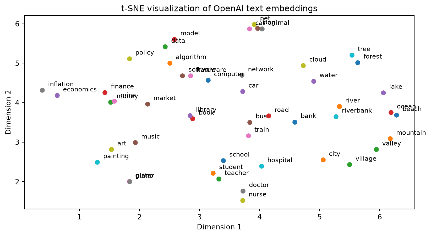
One approach for visualization: come up with a lower-dimensional embedding which approximately preserves local neighborhoods in 2D/3D as in t-SNE (t-Distributed Stochastic Neighbor Embedding)

Get Some Random Embeddings

# Sample a small list of common words and embed them via OpenAIEmbeddings
sampled_tokens = [
  "bank", "river", "money", "finance", "water", "dog", "cat", "animal", "pet", "tree",
  "forest", "city", "village", "road", "car", "bus", "train", "doctor", "nurse", "hospital",
  "school", "student", "teacher", "book", "library", "music", "guitar", "piano", "art", "painting",
  "computer", "algorithm", "data", "model", "economics", "market", "price", "inflation", "policy",
  "riverbank", "beach", "mountain", "valley", "ocean", "lake", "software", "hardware", "network", "cloud"
]
embeddings = embedder.embed_documents(sampled_tokens)  # list[list[float]]
embeddings = np.array(embeddings)
print(f"collected {embeddings.shape[0]} embeddings of dimension {embeddings.shape[1]}")

collected 49 embeddings of dimension 3072

Visualize with t-SNE

tsne = TSNE(n_components=2, random_state=0)  # approx with 2D embedding
embeddings_2d = tsne.fit_transform(embeddings)
# Plot the t-SNE results
plt.figure()
for i, token in enumerate(sampled_tokens):
    x, y = embeddings_2d[i]
    plt.scatter(x, y)
    plt.text(x+0.1, y+0.1, token, fontsize=9)
plt.title('t-SNE visualization of OpenAI text embeddings')
plt.xlabel('Dimension 1')
plt.ylabel('Dimension 2')
plt.show()

Visualize with t-SNE

Sequential Data and Token Prediction

Distribution of Tokens

In many cases, data has an inherent sequential ordering. e.g. time series, language, etc.
Consider conditional probabilities over \(x_t \in \{1, \ldots K\}\). Generically call these “tokens”
Objects of interest: for \(x_1, x_2, \ldots, x_T\) for a sequence of length \(T\) sampled from some population distribution
We may want to condition on the past to predict the next token, condition on the entire sequence to predict missing ones, etc.

Multinomial Logit/Softmax

Often want to map a latent space to a probability distribution over \(K\) outcomes, as the multinomial logit of the classification lecture does
Given a set of \(K\) outcomes, define the logit/softmax mapping a vector \(y \in {\mathbb{R}}^K\) to a probability distribution over \(K\) outcomes as \[ \mathrm{softmax}(y)_k = \frac{e^{y_k}}{\sum_{j=1}^K e^{y_j}}, \quad k = 1, \ldots, K \]
Typically this is combined with a mapping of a latent space, \(z \in {\mathbb{R}}^L\), with some matrix \(W \in {\mathbb{R}}^{K \times L}\) so that \(\mathrm{softmax}(W z)\) is a probability distribution over \(K\) outcomes

\[ \mathbb{P}\left(x = k \,|\, z\right) = \mathrm{softmax}(W z)_k \]

Token Prediction from Conditional Probabilities

Given a sequence \(x_1, x_2, \ldots, x_{t-1}\), model the conditional distribution: \[ \mathbb{P}(x_t | x_{t-1}, x_{t-2}, \ldots, x_1) \]
- Where in the background these are done with marginal and conditional probabilities sampling the population distribution
Basic strategy for sequence models:
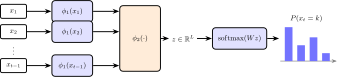
1. Do an embedding for each token \(\phi_1(x_t)\)
2. Map those embeddings to some combined representation, \(\phi_2(\phi_1(x_1), \ldots, \phi_1(x_{t-1}))\)
3. Map that with \(\mathrm{softmax}\) to get probabilities over \(k = 1, \ldots, K\) for \(x_t\)
4. Fit with methods such as maximum likelihood given the multinomial logit structure

From Tokens to the Next-Token Distribution

Embed each token, combine the embeddings into one latent \(z\), and map \(z\) through the softmax to a distribution over the \(K\) possible next tokens

Conditioning on Prior Tokens

The prompt is the conditioning set: the same question after a different history is a draw from a different \(\mathbb{P}(x_t \,|\, x_{t-1}, \ldots, x_1)\)
See Melissa Dell’s Prompting lecture and Prompts for Economists

question = HumanMessage(content="Which meaning of the word bank fits our conversation? One sentence.")
river = [SystemMessage(content="Answer in one sentence."),
         HumanMessage(content="We were talking about fishing on the river."),
         AIMessage(content="Rivers are great places to fish."),
         question]
money = [SystemMessage(content="Answer in one sentence."),
         HumanMessage(content="We were talking about interest rates."),
         AIMessage(content="Interest rates matter for savings."),
         question]
print(f"after river talk: {llm.invoke(river).content}")
print(f"after money talk: {llm.invoke(money).content}")

Conditioning on Prior Tokens

after river talk: In the context of our conversation about fishing on the river, "bank" refers to the land alongside the river where anglers may cast their lines.
after money talk: In our conversation about interest rates, "bank" refers to a financial institution that offers savings accounts and loans.

Mental Model of Sequential Generation

Start with a set of tokens, \(x_1, x_2, \ldots, x_{t-1}\) (include EVERYTHING)
Condition on those tokens to find the \(\mathbb{P}(x_t | x_{t-1}, x_{t-2}, \ldots, x_1)\) distribution
Sample from that to get the \(x_t\) token
- “Temperature” setting mechanically increases/decreases the randomness for the logit (e.g., rescales \(W z\))
Add its own generated token to the set of tokens, \(x_1, x_2, \ldots, x_{t-1}, x_t\)
Condition on those tokens to find the \(\mathbb{P}(x_{t+1} | x_t, x_{t-1}, \ldots, x_1)\) distribution
Repeat until it hits a special “done” token (itself predicted) or reaches a maximum length

Cardinality of the Estimated Conditional Distribution

ChatGPT and others generate text token-by-token auto-regressively
Not directly Markov. \(K^T\) possible sequences of \(K\) tokens of length \(T\)
Modest sized LLMs in 2025 might support \(T=4,000\) with \(K=50,000\) tokens
- Estimating a \(\mathbb{P}: 50,000 \times 50,000^{4,000}\to [0,1]\) conditional PMF
- And growing. Many recent models support \(128k\) tokens for context (i.e., conditioning) and \(16k\) for “output”

How Can This Possibly Work?

It sometimes feels like it has compressed and memorized the entire internet
We don’t always know the parameterization or number of tokens in the training data (remember, this largely uses MLE to train) but OpenAI’s GPT-3 was disclosed
- The \(\mathbb{P}(\cdot | \cdot)\) is approximated by approximating 175 billion parameters
- Trained on 300 billion tokens from close to a terabyte of cleaned text
Which is an absurdly small amount of data given the cardinality of \(\mathbb{P}\)
- Paraphrasing Mikhail Belkin: this is like estimating the Library of Congress with a molecule of ink.