Linear Algebra and Dynamics

Graduate Quantitative Economics and Datascience

Jesse Perla

jesse.perla@ubc.ca

University of British Columbia

Table of contents

• Overview
• Matrix Powers and Eigendecompositions
• Difference Equations
• Steady States and Fixed Points
• Unemployment Dynamics
• PageRank
• Present Discounted Values
• Linearization and StabilityOptional
• ReviewQuestions

Overview

Motivation and Materials

• This lecture applies the tools from the previous one to dynamics in economics and datascience
  • Eigendecompositions to compute matrix powers, and hence the trajectories of linear difference equations
  • Steady states as fixed points, found from eigenvectors or with solve
  • The Neumann series for present discounted values of a stream of payoffs
  • Eigenvectors for the long-run distribution of workers across employment states and of clicks across web pages
  • An optional section on linearizing nonlinear dynamics around a steady state
• The goal is to sharpen your intuition on linear algebra and practice some basic coding

Extra Materials

• Material related to: QuantEcon Python, QuantEcon Data Science, Intro Quantitative Economics with Python
• Self-study and Optional Materials:
  • Geometric Series and Present Values
  • Unemployment Dynamics example
  • Supply and Demand
  • More on Competitive Equilibrium
• For the optional section: Dynamics and Stability in One Dimension, the Solow-Swan Model (skip 20.3), and first-order Taylor expansions

Packages

import numpy as np
import matplotlib.pyplot as plt
from numpy.linalg import matrix_power
from scipy.linalg import inv, solve, eig, eigvals

Matrix Powers and Eigendecompositions

Matrix Powers via the Eigendecomposition

• Iterating a linear map means computing \(A^t = A \cdot A \cdots A\) for large \(t\)
• With the eigendecomposition \(A = Q \Lambda Q^{-1}\), the \(Q^{-1} Q = I\) in the middle cancels

\[ A^2 = (Q \Lambda Q^{-1})(Q \Lambda Q^{-1}) = Q \Lambda (Q^{-1} Q) \Lambda Q^{-1} = Q \Lambda^2 Q^{-1} \]

• Each additional factor of \(A\) cancels the same way, so

\[ A^t = Q \Lambda^t Q^{-1},\quad \Lambda^t = \mathrm{diag}(\lambda_1^t, \ldots, \lambda_N^t) \]

• For symmetric \(A\), \(Q\) is orthogonal so \(Q^{-1} = Q^{\top}\) and \(A^t = Q \Lambda^t Q^{\top}\)

Matrix Powers in NumPy

• Eigenvalues are complex in general. Here they are real, so we drop the zero imaginary parts

A = np.array([[0.9, 0.1],
              [0.5, 0.8]])
Lambda, Q = eig(A)
Lambda = np.real(Lambda)
t = 10
A_t = Q @ np.diag(Lambda**t) @ inv(Q)
print(f"Lambda = {Lambda}")
print(f"Q Lambda^t Q^-1 =\n{A_t}")
print(f"same as A^t? \
{np.allclose(A_t, matrix_power(A, t))}")

Lambda = [1.07912878 0.62087122]
Q Lambda^t Q^-1 =
[[1.30777807 0.46547202]
 [2.3273601  0.84230605]]
same as A^t? True

Difference Equations

Linear Difference Equations as Iterative Maps

• Consider \(A : {\mathbb{R}}^N \to {\mathbb{R}}^N\) as the linear map for the state \(x_t \in {\mathbb{R}}^N\)
• An example of a linear difference equation is

\[ x_{t+1} = A x_t,\quad A \equiv \begin{bmatrix} 0.9 & 0.1 \\ 0.5 & 0.8 \\ \end{bmatrix} \]

x_0 = np.array([1, 1])
x_1 = A @ x_0
print(f"x_1 = {x_1}, x_2 = {A @ x_1}")

x_1 = [1.  1.3], x_2 = [1.03 1.54]

Iterating with \({\varrho\!\left( {A} \right)} > 1\)

Iterate \(x_{t+1} = A x_t\) from \(x_0\) for \(t=200\)

x_0 = np.array([1, 1])
t = 200
x_t = matrix_power(A, t) @ x_0
rho_A = np.max(np.abs(eigvals(A)))
print(f"rho(A) = {rho_A}")
print(f"x_{t} = {x_t}")

rho(A) = 1.079128784747792
x_200 = [3406689.32410673 6102361.18640516]

• Diverges to \(x_{\infty} = \begin{bmatrix} \infty & \infty \end{bmatrix}^{\top}\)
• \({\varrho\!\left( {A} \right)} = 1 + 0.079\) says in the worst case (i.e., \(x_t \propto\) the eigenvector associated with \(\lambda = 1.079\) eigenvalue), expands by \(7.9\%\) on each iteration

Iterating with \({\varrho\!\left( {A} \right)} < 1\)

A = np.array([[0.6, 0.1],
              [0.5, 0.8]])
x_t = matrix_power(A, t) @ x_0
rho_A = np.max(np.abs(eigvals(A)))
print(f"rho(A) = {rho_A}")
print(f"x_{t} = {x_t}")

rho(A) = 0.9449489742783178
x_200 = [6.03450418e-06 2.08159603e-05]

• Converges to \(x_{\infty} = \begin{bmatrix} 0 & 0 \end{bmatrix}^{\top}\)

Eigenvalues Decompose the Dynamics

• Eigenvectors form a basis: so \(x_0 = c_1 q_1 + c_2 q_2\) where \(\begin{bmatrix} c_1 & c_2 \end{bmatrix}^{\top} = Q^{-1} x_0\)
• Then \(x_t = A^t x_0 = c_1 \lambda_1^t q_1 + c_2 \lambda_2^t q_2\): each eigenvector direction scales by its own \(\lambda_i^t\)
  • \({\varrho\!\left( {A} \right)}\) is the fastest-growing direction: \(> 1\) explodes, \(< 1\) decays
  • The smaller \(|\lambda_i|\) is the transient, and its eigenvalue is its decay rate

Lambda, Q = eig(A)
Lambda = np.real(Lambda)
c = solve(Q, x_0) # x_0 = Q c
t = 10
x_t = Q @ (c * Lambda**t)
print(f"Lambda = {Lambda}")
print(f"c = {c}")
print(f"x_{t} = {x_t}")
print(f"same as A^t x_0? \
{np.allclose(x_t, matrix_power(A, t) @ x_0)}")

Lambda = [0.45505103 0.94494897]
c = [-0.88048573 -1.79575746]
x_10 = [0.28401728 0.97878213]
same as A^t x_0? True

Question Initial Conditions

Consider

\[ x_{t+1} = \begin{bmatrix}1.1 & 0 \\ 0 & 0.8\end{bmatrix} x_t, \qquad x_0 = \begin{bmatrix}0 \\ 1\end{bmatrix} \quad\text{or}\quad x_0 = \begin{bmatrix}0.001 \\ 1\end{bmatrix}. \]

Do these two initial conditions produce the same long-run behavior?

Explain without computing matrix powers.

The first trajectory converges to zero: it lies entirely in the eigenvector direction with eigenvalue \(0.8\). The second has a nonzero component in the direction with eigenvalue \(1.1\), which eventually grows without bound.

An expanding direction need not affect every initial condition. The condition \({\varrho\!\left( {A} \right)} < 1\) guarantees convergence to zero from every initial condition.

Steady States and Fixed Points

Affine Difference Equations

• Add a constant: \(x_{t+1} = A x_t + b\) for \(b \in {\mathbb{R}}^N\)
• A steady state \(x^*\) satisfies \(x^* = A x^* + b\), i.e. \((I - A) x^* = b\), a linear system for solve
• Deviations \(\hat{x}_t \equiv x_t - x^*\) follow the homogeneous equation

\[ \hat{x}_{t+1} = A x_t + b - (A x^* + b) = A \hat{x}_t,\quad\text{so}\quad \hat{x}_t = A^t \hat{x}_0 \]

• Hence \(x_t \to x^*\) from any \(x_0\) if and only if \({\varrho\!\left( {A} \right)} < 1\)

b = np.array([1.0, 1.0])
x_star = solve(np.eye(2) - A, b)
x = np.array([1.0, 1.0])
T = 200
for _ in range(T):
    x = A @ x + b
print(f"x_star = {x_star}")
print(f"x_{T} = {x}")

x_star = [10. 30.]
x_200 = [ 9.99989642 29.99964269]

Fixed Points

Fixed Point

Let \(f : S \to S\) for \(S \subseteq {\mathbb{R}}^N\). A fixed point \(x^* \in S\) of \(f\) is one where

\[ x^* = f(x^*) \]

Fixed points may not exist, or there may be several.

• The steady state \(x^* = (I - A)^{-1} b\) is the fixed point of the affine map \(f(x) = A x + b\)
• The linear map \(f(x) = A x\) always has the fixed point \(x^* = 0\)
  • It has others if and only if \(\lambda = 1\) is an eigenvalue: every point on that eigenvector satisfies \(A x^* = x^*\)
  • The next two sections are exactly this case

Infinite Series

Infinite Series

If \({\varrho\!\left( {A} \right)} < 1\) then \(I - A\) is invertible and \((I - A)^{-1} = \sum_{s=0}^{\infty} A^s = I + A + A^2 + \ldots\)

• The matrix version of \(\sum_{s=0}^{\infty} a^s = \frac{1}{1-a}\) for \(|a| < 1\)
• Iterating the affine equation reaches the same steady state as solve: \(x_t = A^t x_0 + \sum_{s=0}^{t-1} A^s b \to (I - A)^{-1} b = x^*\)
• Present discounted values below are the same series with \(\beta A\) in place of \(A\)

A_sum = sum(matrix_power(A, s) for s in range(500))
print(f"sum of A^s =\n{A_sum}")
print(f"inv(I - A) =\n{inv(np.eye(2) - A)}")

sum of A^s =
[[ 6.66666667  3.33333333]
 [16.66666667 13.33333333]]
inv(I - A) =
[[ 6.66666667  3.33333333]
 [16.66666667 13.33333333]]

Question The Largest Eigenvalue

For a diagonalizable matrix \(A\), consider

\[ I + A + A^2 + \cdots, \qquad {\varrho\!\left( {A} \right)} = \max_i |\lambda_i|. \]

Why is checking \({\varrho\!\left( {A} \right)} < 1\) enough for this series to converge?

What happens along the eigenvector direction with the largest \(|\lambda_i|\)?

Along each eigenvector \(q_i\), we have \(A^s q_i = \lambda_i^s q_i\), so the matrix series acts as a scalar geometric series. If the largest \(|\lambda_i|\) is below one, every such series converges. For diagonalizable \(A\), these eigenvectors form a basis.

The eigenvector direction with the largest modulus decays most slowly: effects in that direction persist longest. A negative eigenvalue flips signs, so the absolute value matters. If a unique eigenvalue has the largest modulus and the initial state has a nonzero component along its eigenvector, that component eventually dominates the others. This describes long-run behavior; combinations of nonorthogonal eigenvectors can still grow temporarily.

Unemployment Dynamics

Dynamics of Employment without Population Growth

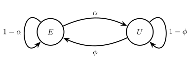
• Consider an economy where in a given year \(\alpha = 5\%\) of employed workers lose job and \(\phi = 10\%\) of unemployed workers find a job
• We start with \(E_0 = 900,000\) employed workers, \(U_0 = 100,000\) unemployed workers, and no birth or death. Dynamics for the year:

\[ \begin{aligned} E_{t+1} &= (1-\alpha) E_t + \phi U_t\\ U_{t+1} &= \alpha E_t + (1-\phi) U_t \end{aligned} \]

Flows Between Employment and Unemployment

• A fraction \(\alpha\) of the employed lose their job and \(\phi\) of the unemployed find one each year
• The same two-state structure returns as a Markov chain in the optional stochastic processes deck

Write as Linear System

• Use matrices and vectors to write as a linear system

\[ \underbrace{\begin{bmatrix} E_{t+1}\\U_{t+1}\end{bmatrix}}_{X_{t+1}} = \underbrace{\begin{bmatrix} 1-\alpha & \phi \\ \alpha & 1-\phi \end{bmatrix}}_{ A} \underbrace{\begin{bmatrix} E_{t}\\U_{t}\end{bmatrix}}_{X_t} \]

Simulating

Simulate by iterating \(X_{t+1} = A X_t\) from \(X_0\) until \(T=100\)

def simulate(A, X_0, T):
    X = np.zeros((2, T+1))
    X[:,0] = X_0
    for t in range(T):
        X[:,t+1] = A @ X[:,t]
    return X
X_0 = np.array([900000, 100000])
A = np.array([[0.95, 0.1], [0.05, 0.9]])
T = 100
X = simulate(A, X_0, T)
print(f"X_{T} = {X[:,T]}")

X_100 = [666666.6870779  333333.31292209]

Dynamics of Unemployment

fig, ax = plt.subplots()
ax.plot(range(T+1), X.T,
  label=["Employed", "Unemployed"])
ax.set(xlabel="t",
  ylabel="Number of Workers",
  title="Employment Status")
ax.legend()
plt.show()

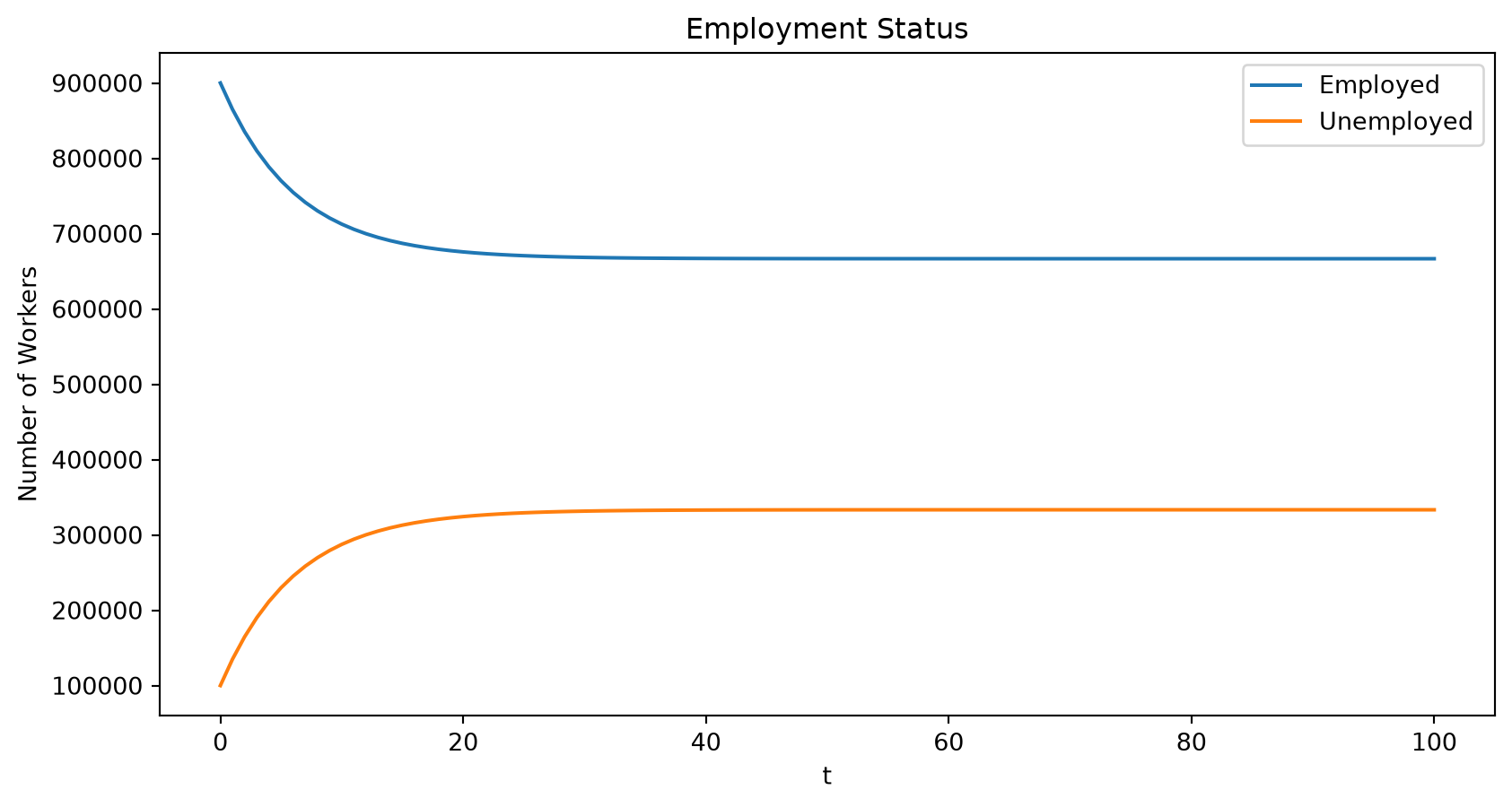
Convergence to a Longrun Distribution

• Find \(X_{\infty}\) by iterating \(X_{t+1} = A X_t\) many times from a \(X_0\)?

  • Check if it has converged with \(X_{\infty} \approx A X_{\infty}\)
  • Is \(X_{\infty}\) the same from any \(X_0\)? The optional stochastic processes deck covers this “ergodicity” question

• Alternatively, note that this expression is the same as

  \[ 1 \times \bar{X} = A \bar{X} \]

  • i.e, a \(\lambda = 1\) where \(\bar{X}\) is the corresponding eigenvector of \(A\), a fixed point of the linear map \(X \mapsto A X\)
  • Is \(\lambda = 1\) always an eigenvalue? (yes if all \(\sum_{n=1}^N A_{ni} = 1\) for all \(i\))
  • Does \(\bar{X} = X_{\infty}\)? For any \(X_0\)?
  • Multiple eigenvalues with \(\lambda = 1 \implies\) multiple \(\bar{X}\)

Using the First Eigenvector for the Steady State

Lambda, Q = eig(A)
print(f"real eigenvalues = {np.real(Lambda)}")
print(f"eigenvectors in columns of =\n{Q}")
print(f"first eigenvalue = 1? \
{np.isclose(Lambda[0], 1.0)}")
X_bar = Q[:,0] / np.sum(Q[:,0]) * np.sum(X_0)
print(f"X_bar = {X_bar}\nX_{T} = {X[:,T]}")

real eigenvalues = [1.   0.85]
eigenvectors in columns of =
[[ 0.89442719 -0.70710678]
 [ 0.4472136   0.70710678]]
first eigenvalue = 1? True
X_bar = [666666.66666667 333333.33333333]
X_100 = [666666.6870779  333333.31292209]

Question Worker Turnover

Suppose both probabilities double:

• Job loss: \(\alpha = 5\% \to 10\%\).
• Job finding: \(\phi = 10\% \to 20\%\).

Does long-run unemployment rise, fall, or stay the same?

Does the economy approach it faster or slower? Explain using worker flows.

Long-run unemployment is unchanged. At the steady state, inflows and outflows balance: \(\alpha E = \phi U\). Doubling both probabilities preserves this balance and the unemployment share \(\alpha/(\alpha+\phi) = 1/3\).

Adjustment is faster: the second eigenvalue \(1-\alpha-\phi\) falls from \(0.85\) to \(0.70\), so deviations from the steady state decay faster. More layoffs need not mean higher long-run unemployment when job finding also increases.

Using the Second Eigenvalue for the Convergence Speed

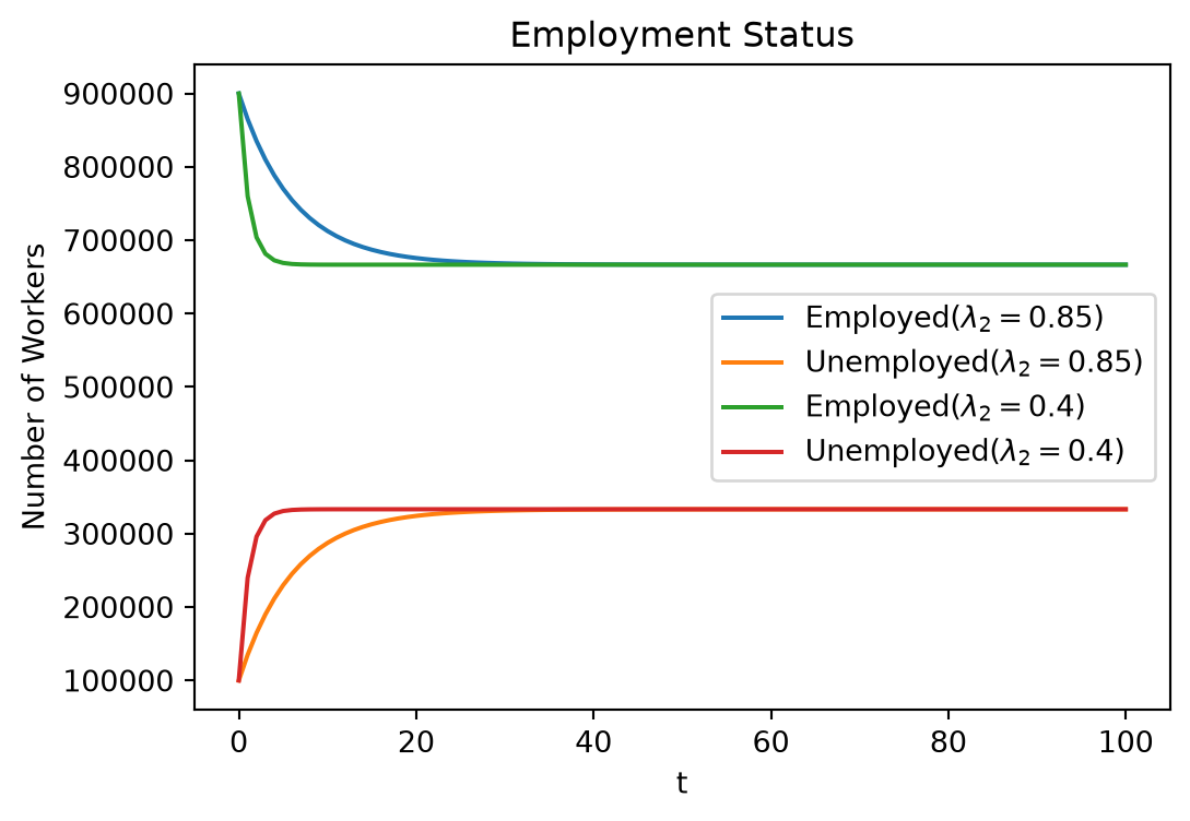
• The second largest (\(\lambda_2 < 1\)) provides information on the speed of convergence
  • \(0\) is instantaneous convergence here
  • \(1\) is no convergence here
• We will create a new matrix with the same steady state, different speed
  • To do this, build a new matrix with the same eigenvectors (in particular the same eigenvector associated with the \(\lambda=1\) eigenvalue)
  • But we will replace the eigenvalues \(\begin{bmatrix}1.0 & 0.85\end{bmatrix}\) with \(\begin{bmatrix}1.0 & 0.4\end{bmatrix}\)
  • Then we will reconstruct \(A\) matrix and simulate again
• Intuitively we will see the that the resulting \(A_{\text{fast}}\) implies \(\alpha\) and \(\phi\) which are larger by the same proportion
• The eigenvector for \(\lambda_2\) sums to zero (it moves workers between \(E\) and \(U\) without changing the total), so \(X_t - \bar{X} \propto \lambda_2^t\) times it: the second eigenvector is the direction of the transient

Simulating with Different Eigenvalues

Lambda_fast = np.array([1.0, 0.4])
A_fast = Q @ np.diag(Lambda_fast) @ inv(Q) # same eigenvectors
print("A_fast =\n", A_fast)
print(f"alpha_fast/alpha = {A_fast[1,0]/A[1,0]:.2g}, \
phi_fast/phi = {A_fast[0,1]/A[0,1]:.2g}")
X_fast = simulate(A_fast, X_0, T)
print(f"X_{T} = {X_fast[:,T]}")

A_fast =
 [[0.8 0.4]
 [0.2 0.6]]
alpha_fast/alpha = 4, phi_fast/phi = 4
X_100 = [666666.66666667 333333.33333333]

Convergence Dynamics of Unemployment

PageRank

Network of Web Pages

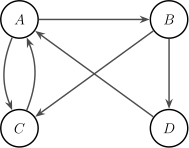
• Consider \(A, B, C, D\) as a set of web pages with links given below
• Which page is the most important? \(A\) and \(C\) each have two links pointing at them

Create an Adjacency Matrix

• We can summarize the network of web pages with \(1\) or \(0\) if there is a link between two pages. Pages won’t link to themselves
• Row \(i\) is the page you are on, column \(j\) is the page linked to, in (arbitrary) order: A, B, C, D

\[ M = \begin{array}{c c l} & \textcolor{gray}{\begin{array}{cccc} A & B & C & D \end{array}} & \\ \textcolor{gray}{\begin{array}{c} A \\ B \\ C \\ D \end{array}} & \begin{bmatrix} 0 & 1 & 1 & 0 \\ 0 & 0 & 1 & 1 \\ 1 & 0 & 0 & 0 \\ 1 & 0 & 0 & 0 \end{bmatrix} & \begin{array}{l} x_t = \textcolor{gray}{A} \;\to\; x_{t+1} = \textcolor{gray}{B} \text{ or } \textcolor{gray}{C} \\ x_t = \textcolor{gray}{B} \;\to\; x_{t+1} = \textcolor{gray}{C} \text{ or } \textcolor{gray}{D} \\ x_t = \textcolor{gray}{C} \;\to\; x_{t+1} = \textcolor{gray}{A} \\ x_t = \textcolor{gray}{D} \;\to\; x_{t+1} = \textcolor{gray}{A} \end{array} \end{array} \]

PageRank Algorithm

One interpretation of this is that you can

• Start on some page
• With equal probability click on all pages linked at that page
• Keep doing this process and then determine what fraction of time you spend on each page

Question Incoming Links

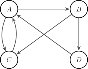
Pages \(A\) and \(C\) each have two incoming links.

If someone keeps clicking randomly among the available links, which page will they spend more time on?

Give an argument from the picture.

Page \(A\): \(C\) and \(D\) send all their traffic to \(A\), while \(A\) and \(B\) split their outgoing traffic. At stationarity, \(r_B = r_A/2\) and \(r_C = r_A/2 + r_B/2 = 3r_A/4\), so \(r_A > r_C\).

The stationary shares are \((r_A,r_B,r_C,r_D) = (0.4,0.2,0.3,0.1)\). Incoming links carry different amounts of traffic; counting them alone misses this.

Probabilistic Interpretation

Alternatively,

• Start with a probability distribution, \(r_t\) that you will be on any given page (i.e. \(r_{nt} \geq 0\) and \(\sum_{n=1}^4 r_{nt} = 1\))
• Iterate the process to see the probability distribution after you click the next links
• Repeat until the probability distribution doesn’t change.

Adjacency Matrix to Probabilities

• To implement, we want to put the same probability on going to any link for a given page (i.e. each row)
• Divide each row of \(M\) by the number of links on that page, so every row of \(S\) sums to one

M = np.array([[0, 1, 1, 0],
              [0, 0, 1, 1],
              [1, 0, 0, 0],
              [1, 0, 0, 0]])
S = M / M.sum(axis=1, keepdims=True)
print(S)

[[0.  0.5 0.5 0. ]
 [0.  0.  0.5 0.5]
 [1.  0.  0.  0. ]
 [1.  0.  0.  0. ]]

Probabilities Evolution

• For a given \(r_t\) distribution of probabilities across pages, the distribution after one more click is

\[ r_{t+1} = S^{\top} r_t \]

• Same structure as the unemployment dynamics: the columns of \(S^{\top}\) sum to one, so \(\lambda = 1\) is an eigenvalue and probability mass is conserved
• Starting on page \(A\) for certain and iterating, the distribution settles down

r_0 = np.array([1.0, 0.0, 0.0, 0.0])
for T in [1, 2, 5, 20]:
    r_T = matrix_power(S.T, T) @ r_0
    print(f"r_{T} = {np.round(r_T, 4)}")

r_1 = [0.  0.5 0.5 0. ]
r_2 = [0.5  0.   0.25 0.25]
r_5 = [0.5   0.125 0.25  0.125]
r_20 = [0.3994 0.2002 0.3003 0.1001]

Long-run Distribution and Eigenvectors

• The stationary distribution \(\bar{r} = S^{\top} \bar{r}\) is a fixed point of \(r \mapsto S^{\top} r\): the eigenvector of \(S^{\top}\) with \(\lambda = 1\), rescaled to sum to one
• The other eigenvalues have \(|\lambda| < 1\), and the largest of them sets the speed of convergence

Lambda, Q = eig(S.T)
i = np.argmin(np.abs(Lambda - 1.0))
r_bar = np.real(Q[:, i])
r_bar = r_bar / np.sum(r_bar)
print(f"|eigenvalues| = {np.round(np.abs(Lambda), 3)}")
print(f"r_bar = {r_bar}")

|eigenvalues| = [1.    0.707 0.707 0.   ]
r_bar = [0.4 0.2 0.3 0.1]

• \(A\) outranks \(C\) even though both have two incoming links: \(C\) and \(D\) link only to \(A\), while \(A\) and \(B\) split their links. A link from an important page, or from a page with few links, counts for more

PageRank at Scale

• The real PageRank is a little more subtle (adds in dampening) but the same basic idea
• With billions of pages, an eigendecomposition is \(O(N^3)\) and infeasible
• Iterating \(r_{t+1} = S^{\top} r_t\) is \(O(N^2)\) per step, and far less since almost every entry of \(S\) is zero. Convergence is geometric at the rate of the second largest \(|\lambda|\)
  • This “power iteration” is exactly what we did by simulating, and is how the eigenvector is found in practice
• Motivation to learn more probability, and Markov chains in the optional stochastic processes deck

Present Discounted Values

Basic Asset Pricing

• Deterministic, infinite horizon, risk-neutral asset pricing based on fundamentals
• Present-value of cashflows, dividends, etc.
• Discount factor \(\beta \in (0,1)\)
  • Might come from consumer impatience, or an internal rate of return
  • Or can get out of risk-free interest rate \(r\) as \(\beta = \frac{1}{1+r}\) in some cases
• Could price based on fundamentals as:

\[ p_t = \sum_{s=0}^{\infty} \beta^s y_{t+s} \]

Scalar Aggregate State

• Assume dividends follow \(y_{t+1} = a y_t\) for \(t=0,1,\ldots\) and \(y_0\) is given

• \(a > 0\) shows how period-payoffs evolve. Can only be a growth or shrinkage factor here.

  \[ p_t = \sum_{s=0}^{\infty} \beta^s y_{t+s} = \frac{y_t}{1-\beta a} \]

  • Note that \(\beta a < 1\) is required for convergence
  • If \(a\) makes dividends grow faster than the discount rate, then the fundamental price is undefined
  • Of course, assets don’t grow forever, but if they grow for a long time this could still be a problem

Geometric Series for Linear State Space Models

• More generally for vector \(x_t\in{\mathbb{R}}^N\) capturing the relevant state of the world for payoff \(y_t\):

  • \(x_{t+1} = A x_t\) with \(y_t = G x_t\)
  • \(A \in {\mathbb{R}}^{N \times N}\) and \(G \in {\mathbb{R}}^{1 \times N}\) then
  • Called a linear state space model

  \[ \begin{aligned} p_t &= y_t + \beta y_{t+1} + \beta^2 y_{t+2} + \ldots = G x_t + \beta G A x_t + \beta^2 G A A x_t + \ldots\\ &= G \sum_{s=0}^{\infty} (\beta A)^s x_t = G (I - \beta A)^{-1} x_t \end{aligned} \]

• The Neumann series with \(\beta A\) requires \({\varrho\!\left( {\beta A} \right)} = \beta {\varrho\!\left( {A} \right)} < 1\): the maximum expansion of \(A\) in its worst direction must be less than the discounting, or the infinite PDV is not defined

• The scalar case is \(A = \begin{bmatrix} a \end{bmatrix}\), \(G = \begin{bmatrix} 1 \end{bmatrix}\) and \({\varrho\!\left( {A} \right)} = a\)

PDV Example

Here is an example with \(1 < {\varrho\!\left( {A} \right)} < 1/\beta\). Try with different \(A\)

beta = 0.9
A = np.array([[0.85, 0.1],
              [0.2, 0.9]])
G = np.array([[1.0, 1.0]]) # row vector
x_0 = np.array([1.0, 1.0])
p_t = G @ solve(np.eye(2) - beta * A, x_0)
#p_t = G @ inv(np.eye(2) - beta * A) @ x_0 # alternative
rho_A = np.max(np.abs(eigvals(A)))
print(f"p_t = {p_t[0]:.4g}, spectral radius = {rho_A:.4g}, \
1/beta = {1/beta:.4g}")

p_t = 24.43, spectral radius = 1.019, 1/beta = 1.111

Linearization and StabilityOptional

Stability of a Fixed Point

• Consider \(x_{t+1} = f(x_t)\) for a possibly nonlinear \(f : {\mathbb{R}}^N \to {\mathbb{R}}^N\) with a fixed point \(x^* = f(x^*)\)
• The Jacobian \(\nabla f(x^*)\) plays the role of \(A\)
  • For the affine \(f(x) = A x + b\) it is exactly \(A\), and \(\hat{x}_t \to 0\) from any \(\hat{x}_0\) if and only if \({\varrho\!\left( {A} \right)} < 1\)
• For nonlinear \(f\) the same condition is local: \(x^*\) is a stable fixed point if \({\varrho\!\left( {\nabla f(x^*)} \right)} < 1\), so small perturbations return to it
  • Necessary but not sufficient globally. \({\varrho\!\left( {\nabla f(x^*)} \right)} > 1 \implies x^*\) can’t be a stable fixed point, but \(< 1\) says nothing about starting far away
• You may see this when working with macro models in Dynare and similar methods in macroeconomics

Linearization

• Assume steady state \(x^* = f(x^*)\) exists, with system \(x_{t+1} = f(x_t)\)
• Take first-order taylor expansion around \(x^*\)

\[ \begin{aligned} x_{t+1} &= f(x^*) + \nabla f(x^*) (x_t - x^*) + \text{second order and smaller terms}\\ x_{t+1} - x^* &\approx \nabla f(x^*) (x_t - x^*)\\ \hat{x}_{t+1} &\approx \nabla f(x^*) \hat{x}_t \end{aligned} \]

• Where the last formulation is common in macroeconomics and time-series econometrics. \(\hat{x}_t\equiv x_t - x^*\) is the deviation from the steady state
  • For the affine case these are exact, as there are no higher-order terms

Quality of Linearization

• Gives approximate dynamics for a perturbation close to the steady state
  • May have good approximation far away from \(x^*\) if \(f(\cdot)\) is close to linear
  • May have terrible approximations close to \(x^*\) if \(f(\cdot)\) highly nonlinear/asymmetric
  • Often log-linearization is used instead, which expresses in percent deviation

Solow-Swan Growth Model

• An early model of economic growth is the Solow-Swan model. We state it rather than derive it; see the link for where the equations come from
  • \(k_t\) is capital per worker, \(z > 0\) is the total factor productivity (TFP)
  • \(\alpha \in (0,1)\) governs the marginal product of capital
  • \(\delta \in (0,1)\) is the depreciation rate, the fraction of machines breaking each year
  • \(s \in (0,1)\) is the fraction of output saved and invested
• Capital follows a nonlinear difference equation

\[ \begin{aligned} k_{t+1} &= s z k_t^{\alpha} + (1-\delta)k_t = s z k_t^{\alpha} + (1-\delta) k_t \equiv g(k_t),\quad \text{ given } k_0 \end{aligned} \]

Steady State and Stability of Solow-Swan

• Fixed point solves \(k^* = g(k^*)\) and hence \(s z k^{*\alpha} = \delta k^*\) and \(k^* = \left(s z/\delta\right)^{1/(1-\alpha)}\)
• Taylor expand \(g\) around \(k^*\), subtract \(k^* = g(k^*)\), then use \(s z k^{*\alpha - 1} = \delta\)

\[ \begin{aligned} k_{t+1} = g(k_t) &\approx g(k^*) + g'(k^*)(k_t - k^*)\\ \underbrace{k_{t+1} - k^*}_{\equiv \hat{k}_{t+1}} &\approx g'(k^*) \underbrace{(k_t - k^*)}_{\equiv \hat{k}_t}\\ \hat{k}_{t+1} &\approx \left(\alpha s z k^{*\alpha-1} + 1-\delta\right) \hat{k}_t = \underbrace{\left(1 - (1-\alpha)\delta\right)}_{\equiv A} \hat{k}_t \end{aligned} \]

Stability

• This is the linear \(\hat{x}_{t+1} = A \hat{x}_t\) with \({\varrho\!\left( {A} \right)} = |1 - (1-\alpha)\delta| < 1\) since \(\alpha, \delta \in (0,1)\)
  • So \(\hat{k}_t \approx A^t \hat{k}_0 \to 0\): \(k^*\) is locally stable for any \(z\) and \(s\)
• Aside: in macroeconomics, industrial organization, etc. this is related to contraction mappings and Blackwell’s condition

Checking Numerically

z, s, alpha, delta = 2, 0.3, 0.3, 0.4
def g(k):
    return s * z * k**alpha + (1 - delta) * k
k_star = (s * z / delta)**(1 / (1 - alpha))
g_prime = alpha * s * z * k_star**(alpha - 1) + 1 - delta
k = 0.25
for _ in range(10):
    k = g(k)
print(f"k_star = {k_star:.4f}, g(k_star) = {g(k_star):.4f}")
print(f"g'(k_star) = {g_prime:.4f} = {1 - (1 - alpha) * delta:.4f}")
print(f"k_10 = {k:.4f}")

k_star = 1.7847, g(k_star) = 1.7847
g'(k_star) = 0.7200 = 0.7200
k_10 = 1.7053

ReviewQuestions

Question Discounting and Convergence

The matrix

\[ A = \begin{bmatrix}0.9 & 0.3 \\ 0.3 & 0.9\end{bmatrix} \quad\text{has eigenvalues}\quad 1.2,\ 0.6. \]

For which of these discount factors does \(\sum_{s=0}^{\infty} \beta^s A^s\) converge?

A. \(\beta = 0.8\) only.
B. \(\beta = 0.9\) only.
C. Both \(\beta = 0.8\) and \(\beta = 0.9\).
D. Neither.

Question Deviations from a Steady State

For \(x_{t+1} = A x_t + b\), let \(x^*\) be a steady state.

Define \(\hat{x}_t = x_t - x^*\). Which recursion is correct?

A. \(\hat{x}_{t+1} = A\hat{x}_t + b\)
B. \(\hat{x}_{t+1} = A\hat{x}_t\)
C. \(\hat{x}_{t+1} = (A-I)\hat{x}_t\)

Question Convergence Speed

Two employment models have the same steady-state shares. Their transition matrices have eigenvalues

\[ A_1:\quad 1,\ 0.9, \qquad A_2:\quad 1,\ 0.4. \]

Which model’s deviations from its steady state decay faster?

A. The model with \(A_1\).
B. The model with \(A_2\).
C. They decay at the same rate because both have an eigenvalue of \(1\).

Question Normalizing PageRank

An eigenvector of \(S^{\top}\) with eigenvalue \(1\) is

\[ q = \begin{bmatrix}2 \\ 1\end{bmatrix}. \]

What stationary probability vector does it represent?

A. \(\bar{r} = \begin{bmatrix}2 & 1\end{bmatrix}^{\top}\)
B. \(\bar{r} = \frac{1}{\sqrt{5}}\begin{bmatrix}2 & 1\end{bmatrix}^{\top}\)
C. \(\bar{r} = \frac{1}{3}\begin{bmatrix}2 & 1\end{bmatrix}^{\top}\)