Least Squares, Uniqueness, and Regularization
Graduate Quantitative Economics and Datascience
Overview
Motivation
- In this section we will use some of the previous tools and discuss concepts on the curvature of optimization problems
- Doing so, we will consider uniqueness in optimization problems in datascience, economics, and ML
- Our key optimization problems to consider will be the quadratic problems than come out of least squares regressions.
- This will provide a foundation for understanding nonlinear objectives since we can think of Hessians are locally quadratic.
Extra Materials
Packages
This section uses the following packages:
First and Second Order Conditions in Optimization
- For univariate unconstrained optimization \(\min_x f(x)\)
- The FONC was \(f'(x) = 0\).
- But this might not be a valid solution! Or there might be many
- The second order condition gives us more information and provides sufficient conditions
- if \(f''(x) > 0\), then \(x\) is a local minimum; if \(f''(x) < 0\), then \(x\) is a local maximum.
- if \(f''(x) = 0\) then there may be multiple solutions (locally)
Related Univariate Concepts
- Recall in your math prep that for a univariate function \(f(x)\), we have:
- \(f(x)\) is convex if \(f''(x) \geq 0\) for all \(x\) in the domain.
- \(f(x)\) is concave if \(f''(x) \leq 0\) for all \(x\) in the domain.
- \(f(x)\) is strictly convex if \(f''(x) > 0\) for all \(x\) in the domain.
- \(f(x)\) is strictly concave if \(f''(x) < 0\) for all \(x\) in the domain.
- We will generalize these concepts for thinking about multivariate functions
- Local behavior, \(x'\) such that \(|x - x'| < \epsilon\), for some \(\epsilon\) “balls”
Definiteness
Reminder: Positive Definite
A = np.array([[3, 1],
              [1, 2]])
# A_eigs = np.real(eigvals(A)) # symmetric matrices have real eigenvalues
A_eigs = eigvalsh(A) # specialized for symmetric/hermitian matrices
print(A_eigs)
is_positive_definite = np.all(A_eigs > 0)
is_positive_semi_definite = np.all(A_eigs >= 0) # or eigvals(A) >= -eps
print(f"pos-def? {is_positive_definite}")
print(f"pos-semi-def? {is_positive_semi_definite}")
[1.38196601 3.61803399]
pos-def? True
pos-semi-def? TrueReminder: Positive Definite
A = np.array([[3, -0.1],
              [-0.1, 2]])
# A_eigs = np.real(eigvals(A)) # symmetric matrices have real eigenvalues
A_eigs = eigvalsh(A) # specialized for symmetric/hermitian matrices
print(A_eigs)
is_positive_definite = np.all(A_eigs > 0)
is_positive_semi_definite = np.all(A_eigs >= 0) # or eigvals(A) >= -eps
print(f"pos-def? {is_positive_definite}")
print(f"pos-semi-def? {is_positive_semi_definite}")
[1.99009805 3.00990195]
pos-def? True
pos-semi-def? TrueReminder: Positive Semi-Definite Matrices
- The simplest positive-semi-definite (but not posdef) matrix is
A_eigs = eigvalsh(np.array([[1, 0],
                            [0, 0]]))
print(A_eigs)
is_positive_definite = np.all(A_eigs > 0)
is_positive_semi_definite = np.all(A_eigs >= 0) # or eigvals(A) >= -eps
print(f"pos-def? {is_positive_definite}")
print(f"pos-semi-def? {is_positive_semi_definite}")
[0. 1.]
pos-def? False
pos-semi-def? TrueNegative Definite Matrices
- Simply swap the inequality. Think of a convex vs. concave function
A = -1 * np.array([[3, -0.1],
                   [-0.1, 2]])
A_eigs = eigvalsh(A)
print(A_eigs)
is_negative_definite = np.all(A_eigs < 0)
is_negative_semi_definite = np.all(A_eigs <= 0) # or eigvals(A) >= -eps
print(f"neg-def? {is_negative_definite}, neg-semi-def? {is_negative_semi_definite}")
[-3.00990195 -1.99009805]
neg-def? True, neg-semi-def? TrueNegative Semi-Definite Matrix
- Semi-definite, but not definite requires the matrix to not be full rank
- At least one zero eigenvalue is necessary and sufficient for a matrix to be singular
A = np.array([[-1, -1],
              [-1, -1]])
A_eigs = eigvalsh(A)
print(A_eigs)
is_negative_definite = np.all(A_eigs < 0)
is_negative_semi_definite = np.all(A_eigs <= 0) # or eigvals(A) >= -eps
print(f"neg-def? {is_negative_definite}, neg-semi-def? {is_negative_semi_definite}")
[-2. 0.]
neg-def? False, neg-semi-def? TrueIndefinite Matrices
- If a matrix has both positive and negative eigenvalues, it is indefinite
- For example,
Quadratic Forms and Second Order Approximations
Applications
- Many useful places for quadratic forms in economics
- Second order approximations of functions (Taylor series) in macro
- Checking sufficient conditions in optimization problems in micro
- Least squares problems in statistics and ML
- Variance decompositions in econometrics
- With nonlinear functions can look at a local quadratic approximation to understand local behavior and sufficiency of solutions
Quadratic Functions in Higher Dimensions
- Recall univariate function \(f(x) = \frac{a}{2} x^2 + b x + c\) for \(x \in \mathbb{R}\).
- General quadratic for \(x \in \mathbb{R}^N\) requires cross-terms (\(a_{12} x_1 x_2, a_{11} x_1^2\) etc.) and linear terms (e.g, \(b_1 x_1, b_2 x_2\))
- An example form is \(f(x) = \frac{1}{2} x^{\top} A x + b^{\top} x + c\)
- For symmetric matrix \(A\), vector \(b\), and scalar \(c\)
- Not unique, but this form gives convenient gradients and Hessians
Gradients of Quadratic Forms
- Univariate: \(f'(x) \equiv \nabla f(x) = a x + b\) and \(f''(x) \equiv \nabla^2 f(x) = a\)
- Multivariate: \(\nabla f(x) = A x + b\) and \(\nabla^2 f(x) = A\)
- \(\nabla f(x)\) is the gradient vector at \(x\)
- \(\nabla^2 f(x)\) is the Hessian matrix at \(x\)
- Quadratic forms are special since the Hessian is constant (not \(x\) dependent)
Necessary and Sufficient Conditions for Optimization
- The FONC of \(\min_{x}\{} x^{\top}A x + b^{\top} x + c\}\) is
- \(\nabla f(x^*) = A x^* + b = \mathbf{0}\)
- If invertible, then \(x^* = -A^{-1} b\), where uniqueness will be related to identification
- Same condition for minimization and maximization?
- Need second order sufficient condition in general to check min vs. max vs. neither
- \(\nabla^2 f(x^*)\) is positive definite for a unique minimum, semi-definite for a minima with local multiplicity where some directions are “flat”
- Replace with negative definite/semi-definite for maxima
- If neither, then not an optimum to a maximization problem (e.g., saddlepoint)
Example of Constructing Quadratic Form
- For \(f(x_1, x_2) = -3 x_1^2 + x_1 x_2 - \tfrac{1}{2} x_2^2 + x_2 + 5\).
- Let \(x \equiv \begin{bmatrix} x_1 \\ x_2 \end{bmatrix}\) and use canonical \(f(x)=\tfrac{1}{2} x^{\top} A x + b^{\top} x + c\).
- Then \(A \equiv \begin{bmatrix} -6 & 1 \\ 1 & -1 \end{bmatrix}\) (negative definite), \(b \equiv \begin{bmatrix} 0 \\ 1 \end{bmatrix}\), and \(c \equiv 5\).
- Gradient: \(\nabla f(x) = A x + b = \begin{bmatrix} -6 x_1 + x_2 \\ x_1 - x_2 + 1 \end{bmatrix}\).
- Hessian: \(\nabla^2 f(x) = A\).
eigs(A) = [-6.1925824 -0.8074176]
neg-def? True
Indefinite Example
- \(f(x_1, x_2) = -3 x_1^2 + x_1 x_2 + x_2 + 5\)
- \(A = \begin{bmatrix} -6 & 1 \\ 1 & 0 \end{bmatrix}\), \(b = \begin{bmatrix} 0 \\ 1 \end{bmatrix}\), and \(c = 5\)
Strict Concavity/Convexity
- Quadratic functions have the same curvature everywhere, so not \(x\) dependent
- Univariate:
- \(a > 0\) is strict convexity
- \(a < 0\) is strict concavity
- \(a = 0\) is linear (neither)
- Multivariate:
- \(A\) is positive definite is strict convexity, \(A\) is negative definite is strict concavity.
- \(A\) is semi-definite weakly convex (maybe strictly in some “directions”)
- And vice-versa for concavity
- Recall that the univariate is nested: \(A = \begin{bmatrix}a\end{bmatrix}\) with eigenvalue \(a\)
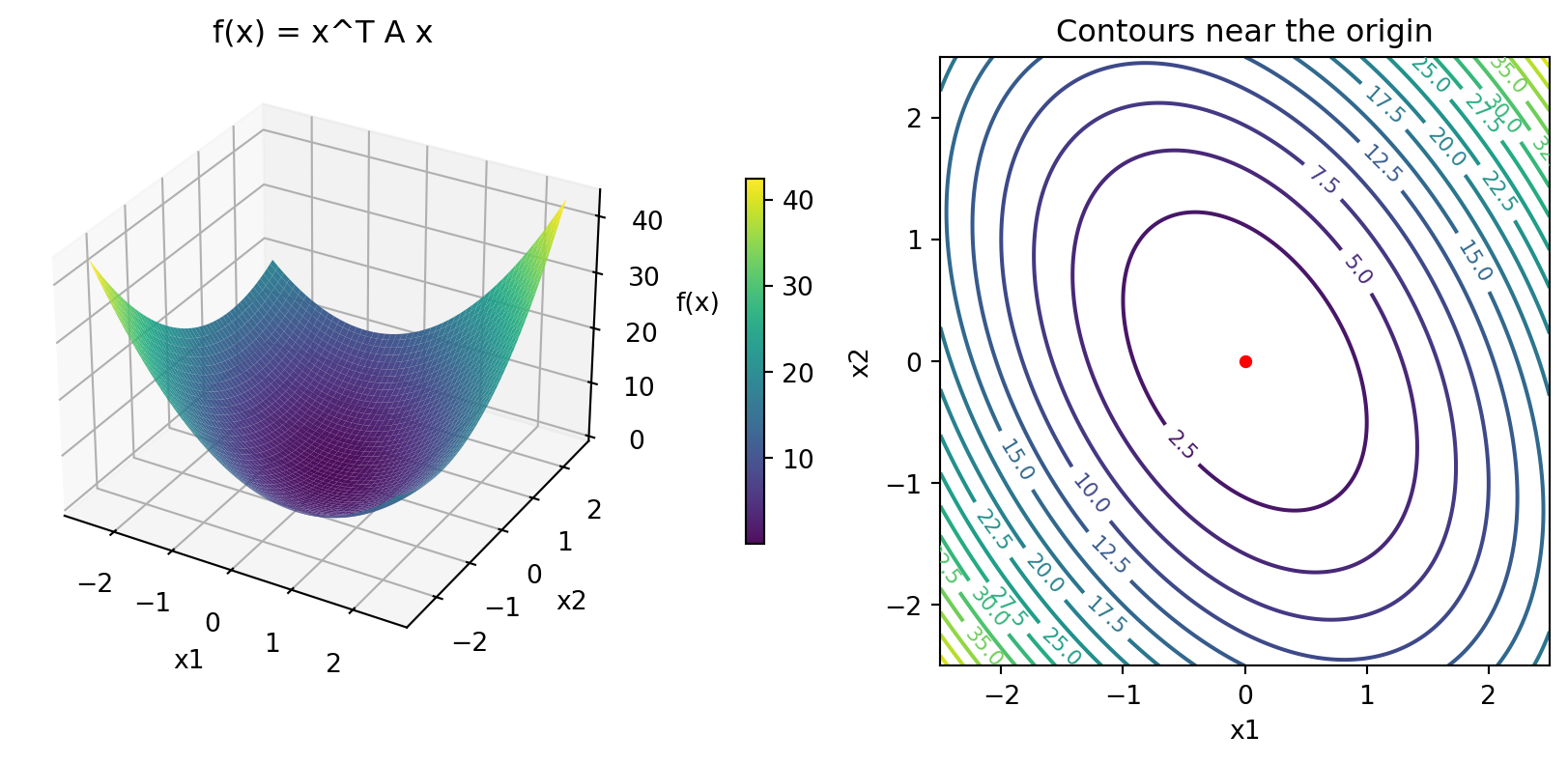
Shape of Positive Definite Function
- For \(A = \begin{bmatrix} 3 & 1 \\ 1 & 2\end{bmatrix}\)
- This has a unique minima (at \((0, 0)\), since no “affine” term, \(b\))
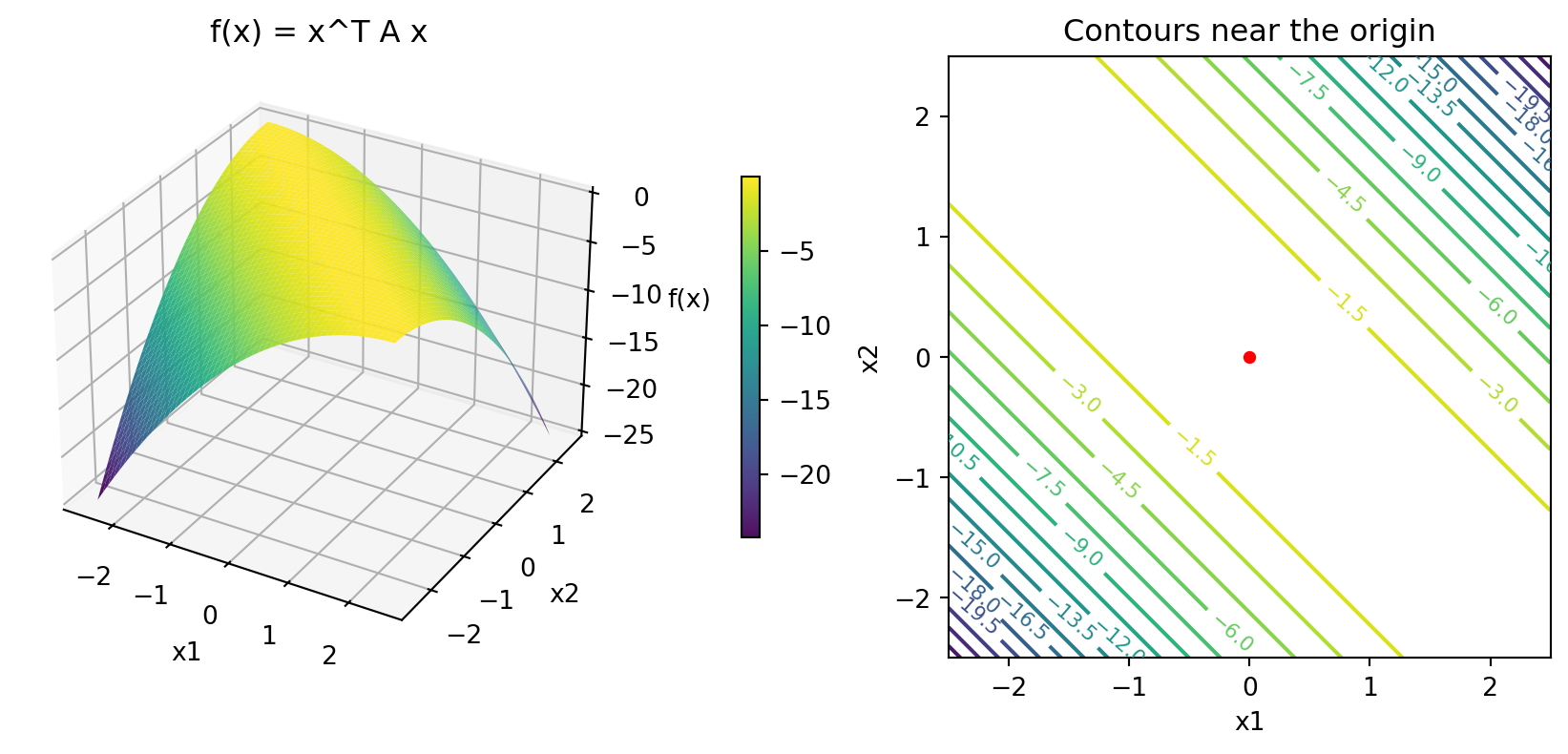
Shape of Negative Semi-Definite Function
- For our \(A = \begin{bmatrix} -1 & -1 \\ -1 & -1\end{bmatrix}\)
- Note that this does not have a unique maximum! All values along a line hold
- Minima rather than maxima since negative rather than positive semi-definite
Shape of an Indefinite Function
- For our \(A = \begin{bmatrix} -6 & 1 \\ 1 & 2\end{bmatrix}\)
- No maxima or minima since indefinite
eigs(A) = [-6.12310563 2.12310563]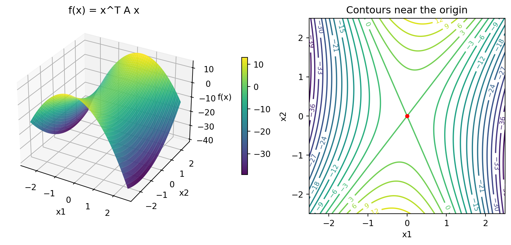
Least Squares and the Normal Equations
Least Squares
Given a matrix \(X \in \mathbb{R}^{N \times M}\) and a vector \(y \in \mathbb{R}^N\), we want to find \(\beta \in \mathbb{R}^M\) such that \[ \begin{aligned} \min_{\beta} &||y - X \beta||^2, \text{ that is,}\\ \min_{\beta} &\sum_{n=1}^N \frac{1}{N}(y_n - X_n \cdot \beta)^2 \end{aligned} \]
Where \(X_n\) is n’th row. Take FOCS and rearrange to get
\[ (X^T X) \beta = X^T y \]
Solving the Normal Equations
The \(X\) is often referred to as the “design matrix”. \(X^T X\) as the Gram matrix
Can form \(A = X^T X\) and \(b = X^T y\) and solve \(A \beta = b\).
- Or invert \(X^T X\) to get
\[ \beta = (X^T X)^{-1} X^T y \]
- Note that \(X^T X\) is symmetric and, if \(X\) is full-rank, positive definite
Solving Regression Models in Practice
lstsqbetter algorithms (more numerically stable, same “order”, possibly slightly slower)- One algorithm uses another factoring, the QR decomposition: \(X = Q R\) for \(Q\) orthogonal and \(R\) upper triangular. See QR Decomposition
- Undergrad suffering through matrix algebra classes: LR decomposition is Gaussian elimination, QR decomposition is Gram-Schmidt orthogonalization
- Stata also uses a \(Q R\) decomposition under the hood.
- For applied work, use Stata, R, or
statsmodels(integrates withpandasandseaborn)- See statsmodels docs for R-style notation and QuantEcon OLS Notes
- For well conditioned problems (i.e., \(\kappa(X^{\top} X)\) small), a Cholesky decomposition on \(X^{\top}X\) then solving \((X^{\top}X) \beta = X^{\top}y\) may be faster but less numerically stable. A useful alternative in some “big data” cases when stata is insufficient.
Example of LLS using Scipy
N, M = 100, 5
X = np.random.randn(N, M)
beta = np.random.randn(M)
y = X @ beta + 0.05 * np.random.randn(N)
beta_hat, residuals, rank, s = scipy.linalg.lstsq(X, y)
print(f"beta =\n {beta}\nbeta_hat =\n{beta_hat}")
beta =
[-0.4342627 1.19270521 -0.4459076 -0.07885572 0.29519551]
beta_hat =
[-0.4276657 1.18800663 -0.43845695 -0.07074571 0.30388576]Solving using the Normal Equations
Or we can solve it directly. Provide matrix structure (so it can use a Cholesky)
XX = X.T @ X
Xy = X.T @ y
beta_hat = solve(XX, Xy, assume_a="pos")
# beta_hat = solve(X.T @ X, X.T @ y, assume_a="pos")
print(f"beta =\n {beta}\nbeta_hat =\n{beta_hat}")
beta =
[-0.4342627 1.19270521 -0.4459076 -0.07885572 0.29519551]
beta_hat =
[-0.4276657 1.18800663 -0.43845695 -0.07074571 0.30388576]Collinearity in “Tall” Matrices
- Tall \(\mathbb{R}^{N\times M}\) “design matrices” have \(N > M\) and are “overdetermined”
- The rank of a matrix is full rank if all columns are linearly independent
- You can only identify \(M\) parameters with \(M\) linearly independent columns
Collinearity and Estimation
- The condition number gets larger with some operations
- If \(X\) is not full rank, then \(X^T X\) is not invertible. For example:
cond(X) = 53.09739144854023, cond(X'*X)=2819.3329786399063, cond(X_col'*X_col)=1.2999933999712892e+16- Note that when you start doing operations on matrices, numerical error creeps in, so you will not get an exact number
- The rule-of-thumb with condition numbers is that if it is \(1\times 10^k\) then you lose about \(k\) digits of precision.
- Given the singular matrix, this means a continuum of \(\beta\) will solve the problem
lstsq Solves it? Careful on Interpretation!
- Since \(X_{col}^T X_{col}\) is singular, we cannot use
solve(X.T@X, y) - But what about
lstsqmethods? - As you will see, this gives an answer. Interpretation is more subtle
- The key is that in the case of non-full rank, you cannot identify individual parameters
- Related to “Identification” in econometrics
- Having low residuals is not enough to conclude anything about identification of parameters
Fat Design Matrices
- Fat \(\mathbb{R}^{N\times M}\) “design matrices” have \(N < M\) and are “underdetermined”
- Less common in econometrics, but useful to understand the structure
- A continuum \(\beta\in\mathbb{R}^{M - \text{rank}(X)}\) solve this problem
Which Solution?
- Residuals are zero here because there are enough parameters to fit perfectly (i.e., it is underdetermined)
- Given the multiple solutions, the
lstsqis giving
\[ \min_{\beta} ||\beta||_2^2 \text{ s.t. } X \beta = y \]
- i.e., the “smallest” coefficients which interpolate the data exactly
- Which trivially fulfills the OLS objective: \(\min_{\beta} ||y - X \beta||_2^2\)
Careful Interpreting Underdetermined Solutions
- Useful and common in ML, but be very careful when interpreting for economics
- Tight connections to Bayesian versions of statistical tests
- But until you understand econometrics and “identification” well, stick to full-rank matrices
- Advanced topics: search for “Regularization”, “Ridgeless Regression” and “Benign Overfitting in Linear Regression.”
Regularization
Recall a Positive Semi-Definite Function
- For our \(A = \begin{bmatrix} 1 & 1 \\ 1 & 1\end{bmatrix}\). Multiple minima along a line!
eigenvalues of A: [2. 0.]
Fudge the Diagonal?
- Replace with \(A = A + \lambda I\) for \(\lambda\) very small (e.g., \(1E-5\))
- Now unique minima at \((0, 0)\)
eigenvalues of A: [2.00001e+00 1.00000e-05]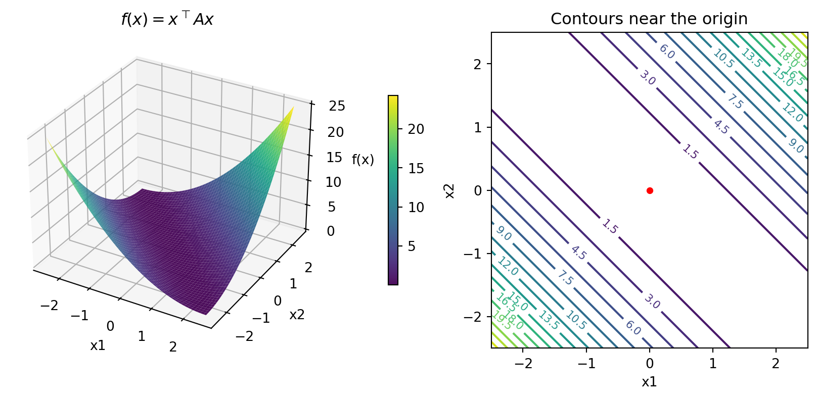
Motivating this Fudge
- Previously solved \(\min_x\left\{x^{\top} A x\right\}\), which only has a unique solution if \(A\) is positive definite.
- Replace with \[
\min_x\left\{x^{\top} A x+ \lambda ||x||_2^2\right\}
\]
- i.e., penalize solutions by the euclidean length of \(x\), called a “ridge” term
- Could instead penalize by different norms, e.g. \(||x||_1\) is called LASSO
- What are the first order conditions? Lets look at least squares
Ridge Regression
- More generally, for OLS think of the following \[ \min_{\beta}\left\{ ||y - X \beta||_2^2 + \lambda ||\beta||_2^2\right\} \]
- Take the FOCs and rearrange to get \[
(X^{\top} X + \lambda I) \beta = X^{\top} y
\]
- Note: if \(X^{\top}X\) is not full rank (i.e., has a zero eigenvalue) then the addition of the \(\lambda\) term helps make things strictly positive definite
- Sometimes you need to do this to overcome nearly collinear data or numerical approximations, even when it should be technically positive definite
Ridgeless Regression
- Recall statement that
lstsqwill return some solution even if not full rank. - We said that in the case where the data could be fit exactly
- One can interpret the solution as \(\min_{\beta} ||\beta||_2^2 \text{ s.t. } X \beta = y\)
- Interpretation: this is the min-norm solution which fits the data with the “smallest” \(\beta\)
- Can show this is the limit of a ridge regression (i.e., “ridgeless”) \[ \lim_{\lambda \to 0}\min_{\beta}\left\{ ||y - X \beta||_2^2 + \lambda ||\beta||_2^2\right\} \]
Regularization in ML
- In ML, with rich data sources there are often many possible ways to explain the data
- Economists often avoid this like the plague, and make assumptions to ensure perfect identification
- Identification arguments ensure positive definiteness of OLS, etc.
- As data becomes richer, it becomes hard to write down models with only a single explanation
- Regularization lets you bias your solution towards ones with certain properties
- There are Bayesian interpretations of all of these approaches
- If you have a strict saddlepoint, then regularization probably isn’t the answe