Latent Variables and Introduction to Unsupervised Learning
Graduate Quantitative Economics and Datascience
Overview
Motivation and Materials
- In this lecture, we will continue with some applications of the tools we developed in the previous lectures
- We introduce scikit-learn, a package for old-school (i.e. not deep learning or neural networks) ML and data analysis
- Introduces “unsupervised learning” (i.e., tools to interpret data structure without any forecasts/predictions)
Extra Materials
Packages
Latent Variables
Features, Labels, and Latents
- Data science and ML often use different terminology than economists:
- Features are economists explanatory or independent variables. They have the key source of variation to make predictions and conduct counterfactuals
- Labels correspond to economists observables or dependent variables
- Latent Variables are unobserved variables, typically sources of heterogeneity or which may drive both the dependent and independent variables
- Economists will use theory and experience to transform data (i.e., what ML people call “feature engineering”) for better explanatory power or map to theoretical models
Unsupervised Learning
- ML refers to methods using only features as unsupervised learning. The structure of the underlying data can teach you about its data generating process
- Key: uncover and interpret latent variables using statistics coupled with assumptions from economic theory. There is theory beyond all interpretation
Principal Components
Principal Components and Factor Analysis
- Another application of eigenvalues is dimension reduction, which simplifies features by uncovering latent variables. Unsupervised
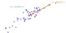
- One technique is Principal Components Analysis (PCA), which uncovers latent variables that capture the primary directions of variation in the underlying data
- May allow mapping data into a lower-dimensional, uncorrelated features
- Uses Singular Value Decomposition (SVD) - a generalization of eigendecomposition to non-square matrices
- Given a matrix \(X \in {\mathbb{R}}^{N \times M}\), can we find a lower-dimensional representation \(Z \in {\mathbb{R}}^{N \times L}\) for \(L < M\) that captures the most variation in \(X\)?
- The goal is to invert the \(X\) data to find the \(Z\)—and provide a mapping to reduce the dimensionality for future data.
Singular Value Decomposition
- Many applications of SVD (e.g., least squares, checking rank), in part because it is especially “numerically stable” (i.e., not sensitive to the roundoff errors we talked about previously)
- One application is to find the latent variables in PCA
- PCA can be interpreted with an eigendecomposition, but can be more confusing than just using the SVD directly.
SVD
An SVD for any \(X \in {\mathbb{R}}^{N\times M}\) is:
\[ X = U \Sigma V^{\top} \]
- The diagonal elements of \(\Sigma \in {\mathbb{R}}^{N\times M}\) are singular values, and there are zeros everywhere else. If \(M < N\) then there are \(M\) singular values (\(\sigma_1, \ldots \sigma_M\))
- Those singular values are also the square roots of the eigenvalues of \(X X^{\top}\) (or \(X^{\top} X\))
- The number of non-zero singular values is the rank of the matrix \(X\)
- \(U\in{\mathbb{R}}^{N\times N}\) and \(V \in {\mathbb{R}}^{M \times M}\) are orthogonal matrices
- \(U\) is eigenvectors of \(X X^{\top}\) and \(V\) is eigenvectors of \(X^{\top} X\)
Decomposing the Data
A key result is that we can decompose the data into a sum of outer products of the eigenvectors and singular values. Assume ordered so that \(\sigma_1 \geq \sigma_2 \geq \ldots \geq \sigma_M\) and \(M \leq N\): \[ X = U \Sigma V^{\top} = \sum_{m=1}^M \sigma_m u_m v_m^{\top} \]
Note that
- \(u_m \in{\mathbb{R}}^N\) is the \(m\)-th column of \(U\) and \(v_m \in{\mathbb{R}}^M\) is the \(m\)th column of \(V\)
- So \(u_m v_m^{\top}\) is an \(N \times M\) matrix but you can show that it is rank-1. i.e., you can decompose it into the product of two vectors.
Interpretation of the Scatter (Covariance) Matrix
- Assuming the data has been de-meaned already, \(X^{\top} X\) is the scatter matrix, i.e. \(N\) times the sample covariance matrix
- The scatter matrix \(X^{\top} X\) is an \(M \times M\) matrix where \[ [X^{\top} X]_{ij} = \sum_{k=1}^N x_{ki} x_{kj} \]
- Calculates an expression related to the covariance between features
- The eigenvectors of this tell you along which directions is there the most variation
Interpretation of the Gram Matrix
- The Gram matrix of the observations (rows) is \(X X^{\top}\), an \(N \times N\) matrix where
\[ [X X^{\top}]_{ij} = x_i^{\top} x_j \]
- i.e., each element measures the similarity between features of the \(i\)th and \(j\)th observations
- Inner products are a classic way to measure similarity
- If \(x_i^{\top} x_j\) is large, then the \(i\)th and \(j\)th observations are similar, and it is maximized if equal.
- If \(x_i^{\top} x_j\) is zero then the observations are orthogonal (uncorrelated once de-meaned)
- This is important in what are called “Kernel methods” which form approximations by comparing the similarity of observations
Interpreting Rank
- Intuition: rank \(r\) if it can be decomposed into the sum of \(r\) rank-1 matrices
- Alternatively, the rank of an \(N \times M\) matrix is \(3\) if we can find a \(A \in {\mathbb{R}}^{N \times 3}\) and \(B \in {\mathbb{R}}^{3 \times M}\) such that \(X = A B\)
- Remember: this works for any matrix \(X \in {\mathbb{R}}^{N \times M}\)
Dimension Reduction
- Frequently \(\sigma_1 \gg \sigma_M\) and the \(\sigma_m\) may decay quickly, so we can approximate \(X\) with fewer terms by truncating the sum at \(L < M\leq N\).
\[ X \approx \sum_{m=1}^L \sigma_m u_m v_m^{\top} \]
- Note that if the data is actually lower-dimensional in a suitable space (e.g., \(\operatorname{rank}(X) = L < M\)) then \(\sigma_m = 0\) for \(L < m \leq M\), so the truncated sum is exact
PCA as an Optimal Dimension Reduction
- Can prove that if we truncate at \(L < M\), this is the best rank \(L\) approximation to \(X\) according to some formal criteria.
- Intuitively, finds directions of the data that capture the most variation in the covariance matrix
- Can prove it is the solution to the optimization problem to explain the most variation in the data with the lowest dimensionality
Creating a Dataset with Latent Factors
Create a dataset with two latent factors, the first dominating
N = 50 # number of observations
L, M = 2, 3 # number of latent and observed factors
Z = np.random.randn(N, L) # latent factors
F = np.array([[1.0, 0.05], # X_1 = Z_1 + 0.05 Z_2
              [2.0, 0.0], # X_2 = 2 Z_1
              [3.0, 0.1]]) # X_3 = 3 Z_1 + 0.1 Z_2
X = Z @ F.T + 0.1 * np.random.randn(N, M) # added noise
print(f"Z is {Z.shape}, X is {X.shape}")
Z is (50, 2), X is (50, 3)PCA Without Dimension Reduction
- See QuantEcon SVD for coding yourself. We will use the sklearn package
- The explained variance is the fraction of the variance explained by each factor
Singular Values (sqrt eigenvalues):
[23.4967  0.7801  0.6799]
Explained Variance (ordered):
[0.9981 0.0011 0.0008]
Dimension Reduction with PCA
pca = PCA(n_components=2) # one less, and correctly specified
Z_hat = pca.fit_transform(X) # transformed by dropping last factor
# Scale and sign may not match due to indeterminacy
print(f"Correlation of Z_1 to Z_hat_1 = {np.corrcoef(Z.T, Z_hat.T)[0,2]}")
print(f"Correlation of Z_2 to Z_hat_2 = {np.corrcoef(Z.T, Z_hat.T)[1,3]}")
Correlation of Z_1 to Z_hat_1 = 0.9991782640019669
Correlation of Z_2 to Z_hat_2 = -0.4829688858606044Interpreting the Results
- The first factor in the decomposition is nearly perfectly (positive or negatively) correlated with the more important latent factor
- The sign could have gone either way. The key is the shared information
- How could you have known the sign is indeterminate?
- The 2nd factor has a good but not great correlation with the 2nd latent. Why?
- The variance decomposition that gave a 3rd factor with non-zero variance
- We only had two latent variables. Why didn’t it figure it out?
- How could you have changed the DGP to make this less successful?
Warning
- We have just scratched the surface to build some intuition.
- Many missing details and caveats (e.g., you may want to rescale your data, make sure everything is demeaned if implementing yourself, etc.)
- Read up on the documentation and theory before using in practice
- Many generalizations exist which are more appropriate in particular settings
Auto-Encoders
Auto-Encoders and Dimensionality Reduction
- General class of problems which they call auto-encoders in ML/data science
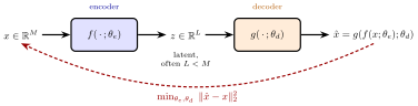
- Function \(f\), the encoder, maps \(X\) to a latent space \(Z\), which may be lower-dimensional
- Function \(g\), the decoder, maps points in the latent space \(Z\) back to \(X\)
- \(\theta_e\) and \(\theta_d\) are parameters for \(f\) and \(g\) which we are trying to find
- Then the goal is to find the \(\theta_e\) and \(\theta_d\) parameters for our encoder, \(f\), and decoder, \(g\), where for as many \(X\) as possible we have
\[ g(f(x; \theta_e); \theta_d) \approx x \]
- The \(z = f(x;\theta_e)\) may be lower-dimensional, but may be useful regardless
Encoder and Decoder
- The encoder compresses \(x\) into the latent \(z\) and the decoder reconstructs \(\hat{x}\); the parameters are chosen so \(\hat{x} \approx x\) across the data
Optimization Problem for an Auto-encoder
If we had a distribution for \(x\) then can solve
\[ \min_{\theta_e, \theta_d} {\mathbb{E}}||g(f(x; \theta_e); \theta_d) - x||_2^2 \]
But typically in practice we replace expectation with empirical distribution \(\{x_1,\ldots x_N\}\)
\[ \min_{\theta_e, \theta_d} \frac{1}{N} \sum_{n=1}^N ||g(f(x_n; \theta_e); \theta_d) - x_n||_2^2 \]
PCA as a Linear Auto-Encoder
- Let \(f(x;W) = W^{\top} x\) and \(g(z;W) = W z\) where \(W \in {\mathbb{R}}^{M \times L}\). If \(\hat{x} \approx W W^{\top} x\), “reconstruction error” is \(||\hat{x} - x||_2^2\).
\[ \min_{W} \frac{1}{N} \sum_{n=1}^N ||W \overbrace{W^{\top} x_n}^{z_n = f(x_n;W)} - x_n||_2^2,\quad \text{with } W^{\top} W = I \]
- In more advanced machine learning examples, intuition seems to come up frequently. Related to embeddings, which come up with NLP, networks, etc.
Connection to PCA
- From a SVD of \(X = U \Sigma V^{\top}\) where \(V\) are the eigenvectors. Assuming \(\Sigma\) is sorted largest to smallest.
- If we are using \(L\) components, then we truncate by taking the first \(L\) columns of \(V\) and \(\Sigma\)
- Then let \(W = V_{1:L}\), so \(W^{\top} W = I\)
- With this, \(f(x) = W^{\top} x\) is a low-dimensional approximation to \(x\) that minimizes the reconstruction error
Discrete Latent Variables
Discrete Latent Variables
- PCA was a way to uncover continuous latent variables or find low-dimensional continuous approximations
- But latent variables may be discrete (e.g., types of people, firms)
- Hidden discrete variables require assigning observations to groups
Clustering
- Clustering lets you take a set of observations with (potentially many) variables (i.e., features) and try to assign a discrete latent variable to each observation
- Theory may or may not help us know the number of groups
- While some are statistical and probabilistic, most methods assign a single latent type rather than a distribution
- Choosing the number of groups to assign to is a challenge that requires theory and regularization - which we will avoid here
- Instead, just as with PCA we will choose the number of groups ad-hoc rather than in a disciplined way
Partitioning Sets
- Let \(X\in{\mathbb{R}}^{N\times M}\) with \(x_1,\ldots x_N\in{\mathbb{R}}^M\) the individual observations
- Assume that each \(x_n\) has a latent discrete \(k \in \{1, \ldots K\}\) then we can assign each observation to one group
- \(\mathbf{S} \equiv \{S_1, \ldots, S_K\}\) where each \(n=1,\ldots N\) is in exactly one \(S_k\) (i.e. a partition)
- The goal is to find the partition which is the most likely to assign each \(x_n\) the correct latent variable \(k\)
- An alternative interpretation is to think of this as a dimension-reduction technique that reduces complicated data into a low-dimensional discrete variable
- In economics, we will sometimes cluster on some observations to reduce the dimension, then leave others continuous
k-means Clustering
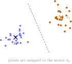
- Consider that the observations \(n \in S_k\) should have similar \(x_n\)
- Group observations that are close or similar to each other
- As always in linear algebra, close suggests using a norm. The Euclidean norm in the \(M\) dimensional feature space is a good baseline
- Objective function of k-means: choose the partition \(\mathbf{S}\) which minimizes the norm between observations within each group
- Normalize by group size \(|S_k|\) to avoid distorting the objective function due to different group sizes
Formal Optimization Problem
Formally,
\[ \min_{\mathbf{S}} \sum_{k=1}^K \frac{1}{2|S_k|}\sum_{x_n, x_{n'} \in S_k} ||x_n - x_{n'}||_2^2 \]
Using standard Euclidean norm between two elements in \(S_k\) \[ ||x_n - x_{n'}||_2^2 = \sum_{m=1}^M (x_{nm} - x_{n'm})^2 \]
k-means Objective Function
Can prove that the previous objective is equivalent to minimizing the sum of the squared distances from the group \(k\)’s mean
\[ \min_{\mathbf{S}} \sum_{k=1}^K \sum_{n \in S_k} ||x_n - \bar{x}_k||_2^2 \]
Where the mean of group \(k\) is standard, and across all \(m\) features
\[ \bar{x}_k \equiv \frac{1}{|S_k|}\sum_{x_n \in S_k} x_n \]
Avoid different scales so \(\bar{x}_k\) isn’t dominated by one feature
Generating Data with Latent Groups
- Generate data with 2 features and 2 latent groups and see how k-means does
- First, put the data in a dataframe
mu_1 = np.array([0.0, 0.0]) # mean of k=1
mu_2 = np.array([1.0, 1.0]) # mean of k=2
sigma = np.array([[0.2, 0], [0, 0.2]]) # use same variance
N = 100 # observations
X_1 = np.random.multivariate_normal(mu_1, sigma, N)
X_2 = np.random.multivariate_normal(mu_2, sigma, N)
df_1 = pd.DataFrame({"f1": X_1[:, 0], "f2": X_1[:, 1], "k": 1})
df_2 = pd.DataFrame({"f1": X_2[:, 0], "f2": X_2[:, 1], "k": 2})
df = pd.concat([df_1, df_2], ignore_index=True)
Plotting Code with Seaborn
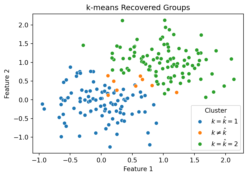
k-means to Recover the Latent Groups
- Run k-means with 2 clusters and check the results
- If correlation is close to 1 then successfully recovered the latent groups
- If the correlation is close to -1 then it was successful. The latent groups \(\hat{k}\) numbers are ordered arbitrarily, just as \(k\) was
Confusion Matrix
- Cross-tabulate the latent \(k\) against the assigned \(\hat{k}\), as in the classification lecture, except that cluster labels are arbitrary
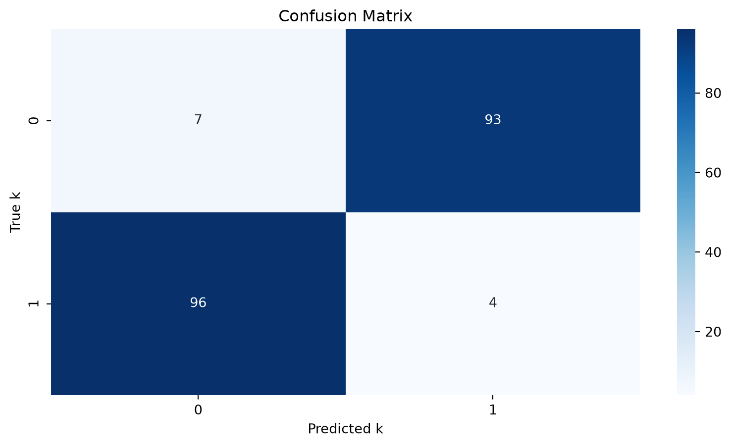
Potentially Swap \(\hat{k}\) and Compare
Label ordering is arbitrary, so the confusion matrix might require reordering to compare
Correlation now 0.8904007705404129Plotting the Uncovered Latent Groups
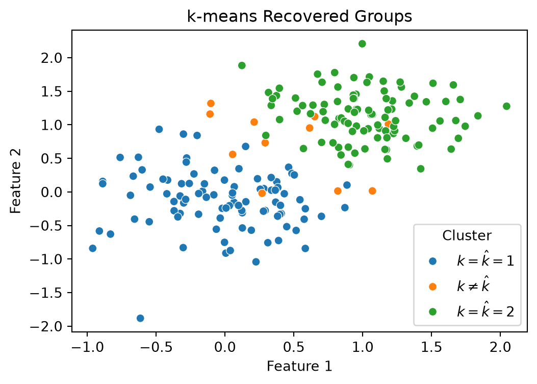
Selecting the Number of Clusters
- A few of the tools people use to help:
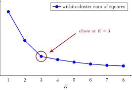
- Elbow method: plot objective function value as a function of \(K\) and look for a kink
- Silhouette method: compute the average distance between points in the same cluster and the nearest cluster
- Cross Validation: split the data and see how well the clustering generalizes
- sklearn docs on silhouette
- The inflection/kink is also useful for choosing the number of components in PCA (Scree plot)
Example of Elbow
- Plot the explained variance as a function of \(K\) for different \(K\)
- When \(K = N\) it must explain 100% of the variance, but kink suggests when marginal improvement slows. See Wikipedia
Art vs. Science
- This is not an endorsement on any of these particular methods.
- Some may be helpful, but there will be some subjectivity and art in most cases
- Ultimately a domain-specific question
Use Economics, and don’t rely on technical tools alone
Factors within a Portfolio ModelOptional
Simulation
In the previous lecture we introduced code for simulation
A Portfolio Example
- Two assets pay dividends \(d_t \equiv \begin{bmatrix} d_{1t} & d_{2t} \end{bmatrix}^{\top}\) following \(d_{t+1} = A\, d_t\) from \(d_0\)
- Portfolio has \(G \equiv \begin{bmatrix} G_1 & G_2 \end{bmatrix}\) shares of each asset and you discount at rate \(\beta\)
A = np.array([[0.6619469, 0.49646018],[0.5840708, 0.4380531]])
G = np.array([[10.0, 4.0]])
d_0 = np.array([1.0, 1.0])
T, beta = 10, 0.9
p_0 = G @ solve(np.eye(2) - beta * A, d_0)
d = simulate(A, d_0, T)
y = G @ d # total dividends from portfolio
print(f"Portfolio value at t=0 is {p_0[0]:.5g}, total dividends at time {T} is {y[0,T]:.5g}")
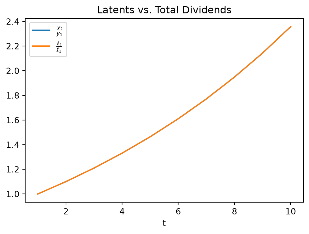
Portfolio value at t=0 is 1424.5, total dividends at time 10 is 36.955Dividends Seem to Grow at a Similar Rate?
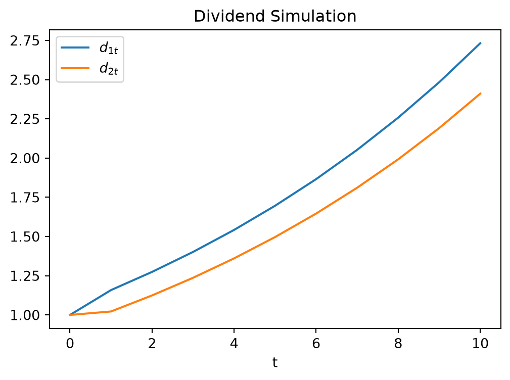
Digging Deeper
- Let’s do an eigendecomposition to analyze the factors
- The first eigenvalue is 1.1, but the second is very close to zero!
- (In fact, I rigged it to be zero by constructing from a \(\Lambda\), so this is all numerical copy/paste errors)
- Suggests that maybe only one latent factor driving both \(d_{1t}\) and \(d_{2t}\)?
- Of course, you may have noticed that the columns in the matrix looked collinear, which was another clue.
Evolution Matrix is Very Simple with \(\lambda_2 = 0\)
If we stack columns \(Q \equiv \begin{bmatrix} q_1 & q_2 \end{bmatrix}\) and let \(\tilde{q}_1\) be the first row of \(Q^{-1}\) then, \[ A = Q \Lambda Q^{-1} = Q \begin{bmatrix} \lambda_1 & 0 \\ 0 & 0 \end{bmatrix} Q^{-1} = \lambda_1 q_1 \tilde{q}_1 \]
Transforming to the Latent State
- Recall: \(A = Q \Lambda Q^{-1}\) can be interpreted as:
- Transformation to latent space, scaling, transform back
- We can demonstrate this in our example:
- Transforming \(d_0\) to \(\ell_0\) using \(\tilde{q}_1\)
- Evolving \(\ell_t\) from \(\ell_0\) with \(\ell_{t+1} = \lambda_1 \ell_t\), or \(\ell_t = \lambda_1^t \ell_0\)
- Transforming back with \(q_1\)
- Checking if it aligns with the \(d_t\)
Implementation
norm = 2.349441087662224e-10Let’s see if these line up perfectly
Total Dividends and the Latent Variable