Applications of Linear Algebra and Eigenvalues
Graduate Quantitative Economics and Datascience
Overview
Motivation and Materials
- In this lecture, we will cover some applications of the tools we developed in the previous lecture
- The goal is to build some useful tools to sharpen your intuition on linear algebra and eigenvalues/eigenvectors, and practice some basic coding
Extra Materials
- Material related to: QuantEcon Python, QuantEcon Data Science, Intro Quantitative Economics with Python
- Self-study and Optional Materials:
Packages
Difference Equations
Linear Difference Equations as Iterative Maps
- Consider \(A : \mathbb{R}^N \to \mathbb{R}^N\) as the linear map for the state \(x_t \in \mathbb{R}^N\)
- An example of a linear difference equation is \[ x_{t+1} = A x_t,\quad A \equiv \begin{bmatrix} 0.9 & 0.1 \\ 0.5 & 0.8 \\ \end{bmatrix} \]
Iterating with \(\rho(A) > 1\)
Iterate \(x_{t+1} = A x_t\) from \(x_0\) for \(t=100\)
rho(A) = 1.079128784747792
x_200 = [3406689.32410673 6102361.18640516]- Diverges to \(x_{\infty} = \begin{bmatrix} \infty & \infty \end{bmatrix}^T\)
- \(\rho = 1 + 0.079\) says in the worst case (i.e., \(x_t \propto\) the eigenvector associated with \(\lambda = 1.079\) eigenvalue), expands by \(7.9\%\) on each iteration
Iterating with \(\rho(A) < 1\)
rho(A) = 0.9449489742783178
x_200 = [6.03450418e-06 2.08159603e-05]- Converges to \(x_{\infty} = \begin{bmatrix} 0 & 0 \end{bmatrix}^T\)
Iterating with \(\rho(A) = 1\)
- To make a matrix that has \(\rho(A) = 1\) reverse eigendecomposition!
- Leave previous eigenvectors in \(Q\), change \(\Lambda\) to force \(\rho(A)\) directly
A = np.array([[0.9, 0.1],
              [0.5, 0.8]]) # rho(A) > 1
Lambda, Q = eig(A)
Lambda = [1.0, 0.8]
A = Q @ np.diag(Lambda) @ inv(Q)
x_t = np.linalg.matrix_power(A, t) @ x_0
print(f"Q =\n{Q}")
print(f"A =\n{A}")
print(f"rho(A) = {np.max(np.abs(eigvals(A)))}")
print(f"x_{t} = {x_t}")
print(f"||x_0|| = {norm(x_0)}")
print(f"||x_{t}|| = {norm(x_t)}")
Q =
[[ 0.48744474 -0.33726692]
[ 0.87315384 0.94140906]]
A =
[[0.92182179 0.04364358]
[0.21821789 0.87817821]]
rho(A) = 1.0
x_200 = [0.82732684 1.48198051]
||x_0|| = 1.4142135623730951
||x_200|| = 1.6972730813998493Stretching?
- Since \(\rho(A) = 1\) we have \(||x_t||\) cannot grow without bound, but \(\lambda_2 < 1\)
- What if we are exactly on the eigenvector associated with \(\lambda_1 = 1\)?
x_0 = [2.04726791 3.66724612]
x_200 = [2.04726791 3.66724612]
||x_0|| = 4.199999999999999
||x_200|| = 4.20000000000001
Disappearing?
- What if we are exactly on the eigenvector associated with \(\lambda_2 = 0.8\)?
- Not sure if there is a useful interpretation of the vector, though.
x_0 = [-1.41652108  3.95391806]
x_200 = [5.53682082e-16 8.72332377e-16]
||x_0|| = 4.2
||x_200|| = 1.0332122842102235e-15
Unemployment Dynamics
Dynamics of Employment without Population Growth
- Consider an economy where in a given year \(\alpha = 5\%\) of employed workers lose job and \(\phi = 10\%\) of unemployed workers find a job
- We start with \(E_0 = 900,000\) employed workers, \(U_0 = 100,000\) unemployed workers, and no birth or death. Dynamics for the year:
\[ \begin{aligned} E_{t+1} &= (1-\alpha) E_t + \phi U_t\\ U_{t+1} &= \alpha E_t + (1-\phi) U_t \end{aligned} \]
Write as Linear System
- Use matrices and vectors to write as a linear system
\[ \underbrace{\begin{bmatrix} E_{t+1}\\U_{t+1}\end{bmatrix}}_{X_{t+1}} = \underbrace{\begin{bmatrix} 1-\alpha & \phi \\ \alpha & 1-\phi \end{bmatrix}}_{ A} \underbrace{\begin{bmatrix} E_{t}\\U_{t}\end{bmatrix}}_{X_t} \]
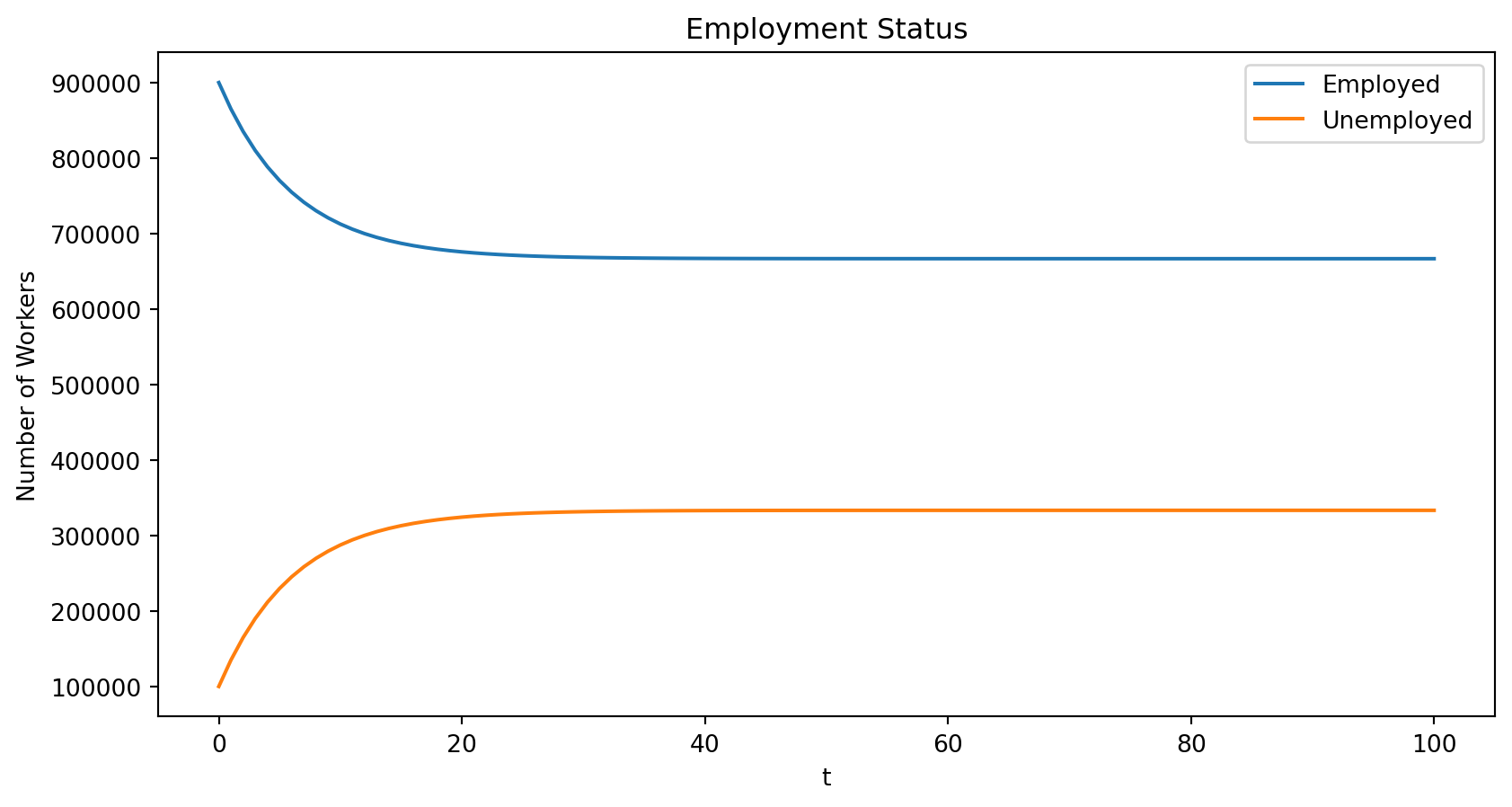
Simulating
Simulate by iterating \(X_{t+1} = A X_t\) from \(X_0\) until \(T=100\)
Dynamics of Unemployment
Convergence to a Longrun Distribution
Find \(X_{\infty}\) by iterating \(X_{t+1} = A X_t\) many times from a \(X_0\)?
- Check if it has converged with \(X_{\infty} \approx A X_{\infty}\)
- Is \(X_{\infty}\) the same from any \(X_0\)? Will discuss “ergodicity” later
Alternatively, note that this expression is the same as
\[ 1 \times \bar{X} = A \bar{X} \]
- i.e, a \(\lambda = 1\) where \(\bar{X}\) is the corresponding eigenvector of \(A\)
- Is \(\lambda = 1\) always an eigenvalue? (yes if all \(\sum_{n=1}^N A_{ni} = 1\) for all \(i\))
- Does \(\bar{X} = X_{\infty}\)? For any \(X_0\)?
- Multiple eigenvalues with \(\lambda = 1 \implies\) multiple \(\bar{X}\)
Using the First Eigenvector for the Steady State
real eigenvalues = [1.   0.85]
eigenvectors in columns of =
[[ 0.89442719 -0.70710678]
 [ 0.4472136   0.70710678]]
first eigenvalue = 1? True
X_bar = [666666.66666667 333333.33333333]
X_100 = [666666.6870779  333333.31292209]
Using the Second Eigenvalue for the Convergence Speed
- The second largest (\(\lambda_2 < 1\)) provides information on the speed of convergence
- \(0\) is instantaneous convergence here
- \(1\) is no convergence here
- We will create a new matrix with the same steady state, different speed
- To do this, build a new matrix with the same eigenvectors (in particular the same eigenvector associated with the \(\lambda=1\) eigenvalue)
- But we will replace the eigenvalues \(\begin{bmatrix}1.0 & 0.85\end{bmatrix}\) with \(\begin{bmatrix}1.0 & 0.5\end{bmatrix}\)
- Then we will reconstruct \(A\) matrix and simulate again
- Intuitively we will see the that the resulting \(A_{\text{fast}}\) implies \(\alpha\) and \(\phi\) which are larger by the same proportion
Simulating with Different Eigenvalues
Lambda_fast = np.array([1.0, 0.4])
A_fast = Q @ np.diag(Lambda_fast) @ inv(Q) # same eigenvectors
print("A_fast =\n", A_fast)
print(f"alpha_fast/alpha = {A_fast[1,0]/A[1,0]:.2g}, \
phi_fast/phi = {A_fast[0,1]/A[0,1]:.2g}")
X_fast = simulate(A_fast, X_0, T)
print(f"X_{T} = {X_fast[:,T]}")
A_fast =
[[0.8 0.4]
[0.2 0.6]]
alpha_fast/alpha = 4, phi_fast/phi = 4
X_100 = [666666.66666667 333333.33333333]Convergence Dynamics of Unemployment
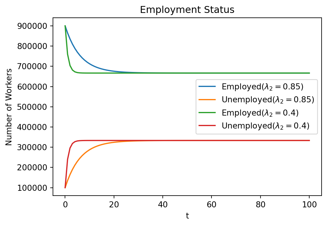
Present Discounted Values
Basic Asset Pricing
- Deterministic, infinite horizon, risk-neutral asset pricing based on fundamentals
- Present-value of cashflows, dividends, etc.
- Discount factor \(\beta \in (0,1)\)
- Might come from consumer impatient, or an internal rate of return
- Or can get out of risk-free interest rate \(r\) as \(\beta = \frac{1}{1+r}\) in some cases
- Could price based on fundamentals as: \[ p_t = \sum_{s=0}^{\infty} \beta^s y_{t+s} \]
Scalar Aggregate State
- Assume dividends follow \(y_{t+1} = a y_t\) for \(t=0,1,\ldots\) and \(y_0\) is given
- \(a > 0\) shows how period-payoffs evolve. Can only be a growth or shrinkage factor here. \[
p_t = \sum_{s=0}^{\infty} \beta^s y_{t+s} = \frac{y_t}{1-\beta a}
\]
- Note that \(\beta a < 1\) is required for convergence
- If \(a\) makes dividends grow faster than the discount rate, then the fundamental price is undefined
- Of course, assets don’t grow forever, but if they grow for a long time this could still be a problem
Geometric Series for LSS
- More generally for vector \(x_t\in\mathbb{R}^N\) capturing the relevant state of the world for payoff \(y_t\):
- \(x_{t+1} = A x_t\) with \(y_t = G x_t\)
- \(A \in \mathbb{R}^{N \times N}\) and \(G \in \mathbb{R}^{1 \times N}\) then
- Called a linear state space model
Convergence
- \(G (I - \beta A)^{-1} x_t\) only has a solution if \(I - \beta A\) is invertible and yields positive \(p_t\)
- Key condition: need spectral radius \(\rho(A) < 1/\beta\)
- Intuition: the spectral radius is the maximum scaling of a vector in the worst possible direction.
- This maximum expansion needs to be less than discounting of the infinite PDV is not defined
- Special case of the scalar case with \(a > 0\)
- \(A = \begin{bmatrix} a \end{bmatrix}\), \(G = \begin{bmatrix} 1 \end{bmatrix}\) and \(\rho(A) = a\)
PDV Example
Here is an example with \(1 < \rho(A) < 1/\beta\). Try with different \(A\)
beta = 0.9
A = np.array([[0.85, 0.1],
              [0.2, 0.9]])
G = np.array([[1.0, 1.0]]) # row vector
x_0 = np.array([1.0, 1.0])
p_t = G @ solve(np.eye(2) - beta * A, x_0)
#p_t = G @ inv(np.eye(2) - beta * A) @ x_0 # alternative
rho_A = np.max(np.abs(np.real(eigvals(A))))
print(f"p_t = {p_t[0]:.4g}, spectral radius = {rho_A:.4g}, 1/beta = {1/beta:.4g}")
p_t = 24.43, spectral radius = 1.019, 1/beta = 1.111