import numpy as np
import matplotlib.pyplot as plt
from numpy.linalg import norm
from scipy.linalg import inv, solve, eig
from sklearn.decomposition import PCADimension Reduction and Continuous Latent Variables
Graduate Quantitative Economics and Datascience
Overview
Motivation and Materials
- Latent variables are unobserved sources of variation, and unsupervised learning uncovers them from the features alone, interpreted with economic theory
- Last lecture the latent variable was discrete: k-means assigned each observation to one of \(K\) groups
- Today the latent variables are continuous: the SVD and PCA find a low-dimensional representation that captures the most variation in the data
- Auto-encoders are the general form of this compression, and the embeddings in the NLP lecture are the next step
- An optional section revisits the eigendecomposition of the dividend model from the dynamics lecture as a one-factor latent
Extra Materials
Packages
Principal Components
Principal Components and Factor Analysis
- Eigenvalues also give us dimension reduction, which simplifies features by uncovering latent variables. Unsupervised
- One technique is Principal Components Analysis (PCA), which uncovers latent variables that capture the primary directions of variation in the underlying data
- May allow mapping data into a lower-dimensional set of uncorrelated features
- Uses Singular Value Decomposition (SVD) - a generalization of eigendecomposition to non-square matrices
- Given a matrix \(X \in {\mathbb{R}}^{N \times M}\), can we find a lower-dimensional representation \(Z \in {\mathbb{R}}^{N \times L}\) for \(L < M\) that captures the most variation in \(X\)?
- The goal is to invert the \(X\) data to find the \(Z\)—and provide a mapping to reduce the dimensionality for future data.
Singular Value Decomposition
- Many applications of SVD (e.g., least squares, checking rank), in part because it is especially “numerically stable” (i.e., not sensitive to the roundoff errors we talked about previously)
- One application is to find the latent variables in PCA
- PCA can be interpreted with an eigendecomposition, but can be more confusing than just using the SVD directly.
SVD
An SVD for any \(X \in {\mathbb{R}}^{N\times M}\) is:
\[ X = U \Sigma V^{\top} \]
- The diagonal elements of \(\Sigma \in {\mathbb{R}}^{N\times M}\) are singular values, and there are zeros everywhere else. If \(M < N\) then there are \(M\) singular values (\(\sigma_1, \ldots \sigma_M\))
- Those singular values are also the square roots of the eigenvalues of \(X X^{\top}\) (or \(X^{\top} X\))
- The number of non-zero singular values is the rank of the matrix \(X\)
- \(U\in{\mathbb{R}}^{N\times N}\) and \(V \in {\mathbb{R}}^{M \times M}\) are orthogonal matrices
- \(U\) is eigenvectors of \(X X^{\top}\) and \(V\) is eigenvectors of \(X^{\top} X\)
Decomposing the Data
A key result is that we can decompose the data into a sum of outer products of the singular vectors and singular values. Assume ordered so that \(\sigma_1 \geq \sigma_2 \geq \ldots \geq \sigma_M\) and \(M \leq N\):
\[ X = U \Sigma V^{\top} = \sum_{m=1}^M \sigma_m u_m v_m^{\top} \]
Note that
- \(u_m \in{\mathbb{R}}^N\) is the \(m\)-th column of \(U\) and \(v_m \in{\mathbb{R}}^M\) is the \(m\)th column of \(V\)
- So \(u_m v_m^{\top}\) is an \(N \times M\) matrix but you can show that it is rank-1. i.e., you can decompose it into the product of two vectors.
Question How Many Nonzero Singular Values?
Build \(X = Z F^{\top}\) with latent \(Z \in {\mathbb{R}}^{N \times 2}\), loadings \(F \in {\mathbb{R}}^{3 \times 2}\), both of full column rank, and no noise, so \(X \in {\mathbb{R}}^{N \times 3}\) with \(N > 3\).
How many nonzero singular values does \(X\) have?
A. \(1\)
B. \(2\)
C. \(3\)
D. \(N\)
- The rank of a product is at most the rank of either factor, and \(Z\) has only \(2\) columns, so \(\operatorname{rank}(X) \leq 2\).
- The number of nonzero singular values is the rank, and full column rank of both factors makes it exactly \(2\).
- Adding noise later makes the third singular value small but nonzero.
Interpretation of the Scatter (Covariance) Matrix
- Assuming the data has been de-meaned already, \(X^{\top} X\) is the scatter matrix, i.e. \(N - 1\) times the usual sample covariance matrix
- The scatter matrix \(X^{\top} X\) is an \(M \times M\) matrix where
\[ [X^{\top} X]_{ij} = \sum_{k=1}^N x_{ki} x_{kj} \]
- Calculates an expression related to the covariance between features
- The eigenvectors of this tell you along which directions is there the most variation
Interpretation of the Gram Matrix
- The Gram matrix of the observations (rows) is \(X X^{\top}\), an \(N \times N\) matrix where
\[ [X X^{\top}]_{ij} = x_i^{\top} x_j \]
- i.e., each element measures the similarity between features of the \(i\)th and \(j\)th observations
- Inner products are a classic way to measure similarity
- If \(x_i^{\top} x_j\) is large, the \(i\)th and \(j\)th observations are large, aligned, or both; for unit-length vectors it is the cosine of the angle between them, maximized when they are equal
- If \(x_i^{\top} x_j\) is zero then the observations are orthogonal
- This is important in what are called “Kernel methods” which form approximations by comparing the similarity of observations
Interpreting Rank
- Intuition: rank \(r\) if \(r\) is the smallest number of rank-1 matrices that sum to it
- Alternatively, the rank of an \(N \times M\) matrix is at most \(3\) if we can find a matrix \(A \in {\mathbb{R}}^{N \times 3}\) and \(B \in {\mathbb{R}}^{3 \times M}\) such that \(X = A B\)
- Remember: this works for any matrix \(X \in {\mathbb{R}}^{N \times M}\)
Dimension Reduction
- Frequently \(\sigma_1 \gg \sigma_M\) and the \(\sigma_m\) may decay quickly, so we can approximate \(X\) with fewer terms by truncating the sum at \(L < M\leq N\).
\[ X \approx \sum_{m=1}^L \sigma_m u_m v_m^{\top} \]
- Note that if the data is actually lower-dimensional in a suitable space (e.g., \(\operatorname{rank}(X) = L < M\)) then \(\sigma_m = 0\) for \(L < m \leq M\), so the truncated sum is exact
- Choose \(L\) from a Scree plot of the \(\sigma_m\) against \(m\): look for the kink, as with the elbow for k-means in the last lecture
PCA as an Optimal Dimension Reduction
- Can prove that if we truncate at \(L < M\), this is the best rank \(L\) approximation to \(X\) according to some formal criteria.
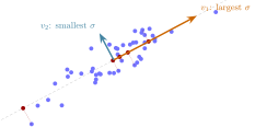
- Intuitively, finds directions of the data that capture the most variation in the covariance matrix
- Can prove it is the solution to the optimization problem to explain the most variation in the data with the lowest dimensionality
Creating a Dataset with Latent Factors
Create a dataset with two latent factors, the first dominating
N = 50 # number of observations
L, M = 2, 3 # number of latent factors and observed features
np.random.seed(77)
Z = np.random.randn(N, L) # latent factors
F = np.array([[1.0, 0.05], # X_1 = Z_1 + 0.05 Z_2
              [2.0, 0.0], # X_2 = 2 Z_1
              [3.0, 0.1]]) # X_3 = 3 Z_1 + 0.1 Z_2
X = Z @ F.T + 0.1 * np.random.randn(N, M) # added noise
print(f"Z is {Z.shape}, X is {X.shape}")
Z is (50, 2), X is (50, 3)PCA Without Dimension Reduction
- See QuantEcon SVD for coding yourself. We will use the sklearn package
- The explained-variance ratio is the fraction of the variance explained by each factor
Singular Values (sqrt eigenvalues):
[24.644   0.8199  0.6185]
Explained Variance Ratio (ordered):
[0.9983 0.0011 0.0006]
Dimension Reduction with PCA
pca = PCA(n_components=2) # one less, and correctly specified
Z_hat = pca.fit_transform(X) # transformed by dropping last factor
# Sign is arbitrary, and the components can mix the latent factors
print(f"Correlation of Z_1 to Z_hat_1 = {np.corrcoef(Z.T, Z_hat.T)[0,2]}")
print(f"Correlation of Z_2 to Z_hat_2 = {np.corrcoef(Z.T, Z_hat.T)[1,3]}")
Correlation of Z_1 to Z_hat_1 = 0.999329900857125
Correlation of Z_2 to Z_hat_2 = -0.479077909271834Question Which Is Also an SVD?
\(X = U \Sigma V^{\top}\) is an SVD of \(X\).
Which change leaves it a valid SVD of the same \(X\)?
A. Flip the sign of \(u_1\) only
B. Double \(\sigma_1\) and halve \(u_1\)
C. Swap \(u_1\) with \(u_2\) only
D. Flip the signs of \(u_1\) and \(v_1\) together
- \(\sigma_1 (-u_1)(-v_1)^{\top} = \sigma_1 u_1 v_1^{\top}\), and both matrices stay orthogonal.
- Flipping \(u_1\) alone changes the sign of the first term, halving \(u_1\) breaks \(\|u_1\|_2 = 1\), and swapping \(u_1\) alone pairs \(u_2\) with \(v_1\).
- So each column of \(\hat{Z}\) from PCA has an arbitrary sign: a correlation of \(-1\) with the true latent is as good as \(+1\).
Interpreting the Results
- The first factor in the decomposition is nearly perfectly (positively or negatively) correlated with the more important latent factor
- The sign could have gone either way. The key is the shared information
- The 2nd factor has only a moderate correlation with the 2nd latent. Why?
- The variance decomposition gave a 3rd factor with non-zero variance
- We only had two latent variables. Why didn’t it figure it out?
- How could you have changed the DGP to make this less successful?
Question Change the Units of One Feature
The data are demeaned and the three features have similar variances. Feature \(3\) switches from dollars to cents, so its column is multiplied by \(100\).
What happens to the first principal direction \(v_1\)?
A. Unchanged; only \(\sigma_1\) changes
B. Tilts away from feature \(3\)
C. Tilts toward feature \(3\)
D. Unchanged because the data are demeaned
- The off-diagonal entries of \(X^{\top} X\) involving feature \(3\) scale by \(100\) and its variance by \(10{,}000\), so that feature dominates the scatter matrix and \(v_1\) rotates toward it. Had \(v_1\) already pointed along feature \(3\), it would barely move and only \(\sigma_1\) would change.
- PCA is not scale invariant. Standardize the features unless their units are comparable.
Warning
- We have just scratched the surface to build some intuition.
- Many missing details and caveats (e.g., you may want to rescale your data, make sure everything is demeaned if implementing yourself, etc.)
- Read up on the documentation and theory before using in practice
- Many generalizations exist which are more appropriate in particular settings
Auto-Encoders
Auto-Encoders and Dimensionality Reduction
- General class of problems which they call auto-encoders in ML/data science
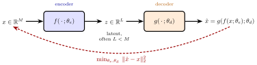
- Function \(f\), the encoder, maps \(X\) to a latent space \(Z\), which may be lower-dimensional
- Function \(g\), the decoder, maps points in the latent space \(Z\) back to \(X\)
- \(\theta_e\) and \(\theta_d\) are parameters for \(f\) and \(g\) which we are trying to find
- Then the goal is to find the \(\theta_e\) and \(\theta_d\) parameters for our encoder, \(f\), and decoder, \(g\), where for as many \(X\) as possible we have
\[ g(f(x; \theta_e); \theta_d) \approx x \]
- The \(z = f(x;\theta_e)\) may be lower-dimensional, but may be useful regardless
Encoder and Decoder
- The encoder compresses \(x\) into the latent \(z\) and the decoder reconstructs \(\hat{x}\); the parameters are chosen so \(\hat{x} \approx x\) across the data
Optimization Problem for an Auto-encoder
If we had a distribution for \(x\) then can solve
\[ \min_{\theta_e, \theta_d} {\mathbb{E}}\|g(f(x; \theta_e); \theta_d) - x\|_2^2 \]
But typically in practice we replace expectation with empirical distribution \(\{x_1,\ldots x_N\}\)
\[ \min_{\theta_e, \theta_d} \frac{1}{N} \sum_{n=1}^N \|g(f(x_n; \theta_e); \theta_d) - x_n\|_2^2 \]
PCA as a Linear Auto-Encoder
- With \(x\) demeaned, let \(f(x;W) = W^{\top} x\) and \(g(z;W) = W z\) where \(W \in {\mathbb{R}}^{M \times L}\). Then \(\hat{x} = W W^{\top} x\) and the “reconstruction error” is \(\|\hat{x} - x\|_2^2\).
\[ \min_{W} \frac{1}{N} \sum_{n=1}^N \|W \overbrace{W^{\top} x_n}^{z_n = f(x_n;W)} - x_n\|_2^2,\quad \text{with } W^{\top} W = I \]
- In more advanced machine learning examples, intuition seems to come up frequently. Related to embeddings, which come up with NLP, networks, etc.
Connection to PCA
- From a SVD of \(X = U \Sigma V^{\top}\) where the columns of \(V\) are the eigenvectors of \(X^{\top} X\). Assuming \(\Sigma\) is sorted largest to smallest.
- If we are using \(L\) components, then we truncate by taking the first \(L\) columns of \(V\) and \(\Sigma\)
- Then let \(W = V_{1:L}\), so \(W^{\top} W = I\)
- With this, \(z = W^{\top} x\) is the low-dimensional latent and \(W z = W W^{\top} x\) the reconstruction that minimizes the error
Question What Does an Auto-Encoder Compare?
An auto-encoder is trained on data \(x_1, \ldots, x_N\).
What does its loss compare?
A. The reconstruction \(\hat{x} = g(f(x))\) to \(x\) itself
B. The latent \(z = f(x)\) to \(x\)
C. The reconstruction \(\hat{x}\) to some label \(y\)
- The data are their own target: the loss is \(\|g(f(x)) - x\|_2^2\), which is why no labels are needed and the method is unsupervised.
- The latent \(z\) is a by-product, usually lower-dimensional than \(x\), and is what we keep. PCA is the linear case with \(W^{\top} W = I\).
Review QuestionsQuestions
Question Remove the Noise
The PCA example in this lecture used \(X = Z F^{\top} + 0.1\, \varepsilon\) with latent \(Z \in {\mathbb{R}}^{50 \times 2}\), loadings \(F \in {\mathbb{R}}^{3 \times 2}\), and Gaussian noise \(\varepsilon\), and PCA gave a third explained-variance ratio of \(0.0006\).
Set the noise to zero, so \(X = Z F^{\top}\) exactly, and refit PCA(n_components=3).
What is the third explained-variance ratio?
A. Zero up to roundoff
B. About \(0.0006\), as before
C. Undefined: PCA fails on a rank-deficient matrix
D. Depends on \(N\)
- \(X\) has rank \(2\), so \(\sigma_3 = 0\) and its share of the variance is \(0\), up to roundoff near \(10^{-16}\).
- The nonzero third component in that example is the \(0.1\, \varepsilon\) noise, which has full rank.
- PCA runs fine on rank-deficient data; it is the inverse in least squares that needs care.
Question Explained Variance Adds Up
Fit PCA(n_components=M) on \(X \in {\mathbb{R}}^{N \times M}\).
What does explained_variance_ratio_ sum to?
A. \(\sigma_1\)
B. \(M\)
C. \(1\)
D. \(N\)
- Component \(m\) explains the share \(\sigma_m^2 / \sum_{j=1}^M \sigma_j^2\), and with all \(M\) components the shares sum to \(1\).
- With
n_components=Lfor \(L < M\) the sum is the share of variance the truncation keeps.
Question No Bottleneck
An auto-encoder has latent dimension \(L = M\), and \(f\) and \(g\) can be any functions.
What is the smallest reconstruction error it can reach?
A. The sum of the smallest singular values
B. Never zero, because of noise in the data
C. Zero, with \(f\) and \(g\) both the identity
D. It depends on the data
- With \(z = x\) and \(\hat{x} = z\), every observation is reconstructed exactly, so the error is \(0\) and nothing about the data is learned.
- The bottleneck \(L < M\) is the whole point: with \(f\) and \(g\) restricted, e.g. linear, it forces the encoder to keep only the directions that matter most for rebuilding \(x\).
Question Ten Ratios, Two Factors
Ten financial ratios per firm are linear combinations of two latent factors of comparable importance, plus noise well below both.
What do the singular values of the demeaned ratio matrix look like?
A. Two large, eight near zero
B. All about the same size
C. One large, nine near zero
D. Decaying at a constant rate
- Without noise the matrix has rank \(2\); small noise lifts the other eight singular values slightly above zero.
- That gap is what a scree plot shows, and it is the evidence that \(L = 2\) is the right truncation.
Question Which Tool for Which Latent?
Three tasks:
- Compress \(50\) balance-sheet ratios per firm into a few indices
- Sort firms into a handful of types
- Find the common factor driving two dividend series with \(d_{t+1} = A\, d_t\)
Which tool fits each?
A. k-means, PCA, eigendecomposition of \(A\)
B. PCA, k-means, eigendecomposition of \(A\)
C. PCA, eigendecomposition of \(A\), k-means
D. k-means for all three
- A continuous low-dimensional latent is PCA; a discrete latent is k-means from the last lecture.
- In the rank-one example of the optional section that follows, the latent is \(\ell_t = \tilde{q}_1 d_t\) and \(q_1\) maps it back into dividends: the eigendecomposition separates the dynamic modes.
Factors within a Portfolio ModelOptional
Simulation
In the dynamics lecture we introduced code for simulation
A Portfolio Example
- Two assets pay dividends \(d_t \equiv \begin{bmatrix} d_{1t} & d_{2t} \end{bmatrix}^{\top}\) following \(d_{t+1} = A\, d_t\) from \(d_0\)
- Portfolio has \(G \equiv \begin{bmatrix} G_1 & G_2 \end{bmatrix}\) shares of each asset and you discount with factor \(\beta\)
A = np.array([[0.6619469, 0.49646018],[0.5840708, 0.4380531]])
G = np.array([[10.0, 4.0]])
d_0 = np.array([1.0, 1.0])
T, beta = 10, 0.9
p_0 = G @ solve(np.eye(2) - beta * A, d_0)
d = simulate(A, d_0, T)
y = G @ d # total dividends from portfolio
print(f"Portfolio value at t=0 is {p_0[0]:.5g}, "
      f"total dividends at time {T} is {y[0,T]:.5g}")
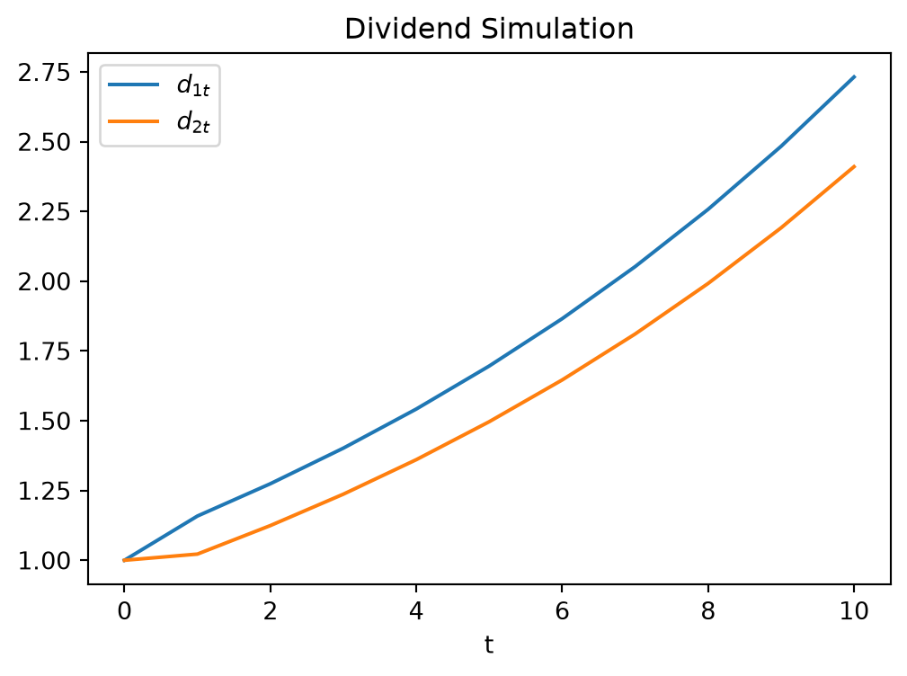
Portfolio value at t=0 is 1424.5, total dividends at time 10 is 36.955Dividends Seem to Grow at a Similar Rate?
Digging Deeper
- Let’s do an eigendecomposition to analyze the factors
- The first eigenvalue is 1.1, but the second is very close to zero!
- (In fact, I rigged it to be zero by constructing from a \(\Lambda\), so this is all numerical copy/paste errors)
- Suggests that maybe only one latent factor driving both \(d_{1t}\) and \(d_{2t}\)?
- Of course, you may have noticed that the columns in the matrix looked collinear, which was another clue.
Evolution Matrix is Very Simple with \(\lambda_2 = 0\)
If we stack columns \(Q \equiv \begin{bmatrix} q_1 & q_2 \end{bmatrix}\) and let \(\tilde{q}_1\) be the first row of \(Q^{-1}\) then,
\[ A = Q \Lambda Q^{-1} = Q \begin{bmatrix} \lambda_1 & 0 \\ 0 & 0 \end{bmatrix} Q^{-1} = \lambda_1 q_1 \tilde{q}_1 \]
Transforming to the Latent State
- Recall: \(A = Q \Lambda Q^{-1}\) can be interpreted as:
- Transformation to latent space, scaling, transform back
- We can demonstrate this in our example:
- Transforming \(d_0\) to \(\ell_0\) using \(\tilde{q}_1\)
- Evolving \(\ell_t\) from \(\ell_0\) with \(\ell_{t+1} = \lambda_1 \ell_t\), or \(\ell_t = \lambda_1^t \ell_0\)
- Transforming back with \(q_1\)
- Checking if it aligns with the \(d_t\)
Implementation
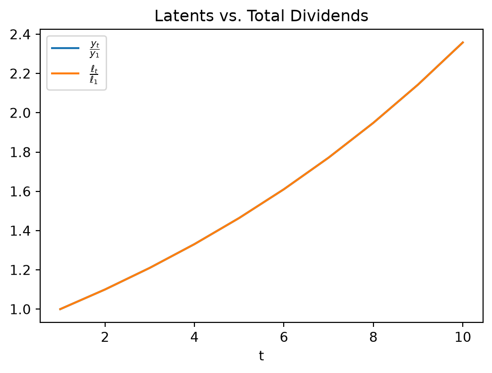
norm = 2.349441087662224e-10Let’s see if these line up perfectly
Total Dividends and the Latent Variable