Classification

Graduate Quantitative Economics and Datascience

Jesse Perla

University of British Columbia

Overview

Motivation

  • Least squares predicts a continuous \(y\). Classification predicts a discrete one: a category, a yes/no, a code
  • Supervised learning: every training observation carries a label \(y_n\). The next lecture is the unsupervised case, features with no labels
  • Economists use classifiers two ways: the outcome itself is discrete (labor force participation, loan approval), or the classifier builds a variable that then enters a regression (an occupation code from a job title, a topic from text)
  • The second use has an econometric consequence: the classifier’s mistakes are measurement error in the generated variable, and its confusion matrix tells you how much

Extra Materials

Packages

import os
import numpy as np
import pandas as pd
import matplotlib.pyplot as plt
from scipy.special import expit
from sklearn.linear_model import LogisticRegression
from sklearn.model_selection import train_test_split
from sklearn.metrics import (confusion_matrix, ConfusionMatrixDisplay,
                             precision_score, recall_score, roc_auc_score,
                             RocCurveDisplay)
from sklearn.feature_extraction.text import CountVectorizer
import statsmodels.api as sm
import statsmodels.formula.api as smf

From Least Squares to Logistic Regression

The Linear Probability Model

  • With \(y_n \in \{0, 1\}\), \({\mathbb{E}}[y_n \,|\, x_n] = \mathbb{P}(y_n = 1 \,|\, x_n)\), so why not least squares?

\[ \mathbb{P}(y_n = 1 \,|\, x_n) = x_n^{\top} \beta \]

  • Fine for a quick look at average effects, and \(\beta_j\) is directly the change in the probability
  • But fitted values can be below \(0\) or above \(1\), and a unit change in \(x_j\) has the same effect whether the probability starts at \(0.5\) or \(0.99\)
  • We want a model whose output is a probability, then a rule that turns it into a class

The Sigmoid

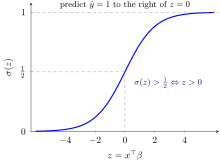
  • The sigmoid maps \({\mathbb{R}}\) to \((0, 1)\); in scipy it is expit

\[ \sigma(z) = \frac{1}{1 + e^{-z}} \]

  • Its inverse is the log-odds, \(\log \frac{p}{1 - p} = z\)
  • Logistic regression puts the linear index inside it

\[ \mathbb{P}(y_n = 1 \,|\, x_n) = \sigma(x_n^{\top} \beta) \]

  • \(\beta_j\) is the effect of \(x_j\) on the log-odds
The Likelihood

  • Each \(y_n\) is Bernoulli with \(p_n \equiv \sigma(x_n^{\top} \beta)\), so

\[ \ell(\beta) = \sum_{n=1}^N \left[ y_n \log p_n + (1 - y_n) \log\left(1 - p_n\right) \right] \]

  • ML calls \(-\ell(\beta)/N\) the cross-entropy or log loss. Minimizing it is maximizing the likelihood
  • With \(\sigma'(z) = \sigma(z)(1 - \sigma(z))\),

\[ \nabla \ell(\beta) = \sum_{n=1}^N (y_n - p_n)\, x_n, \qquad \nabla^2 \ell(\beta) = -\sum_{n=1}^N p_n (1 - p_n)\, x_n x_n^{\top} \]

  • As in least squares the gradient is residual times \(x_n\), but \(p_n\) is nonlinear in \(\beta\)

A Concave Problem

  • The Hessian is \(-X^{\top} W X\) with \(W = \mathrm{diag}(p_1 (1 - p_1), \ldots, p_N (1 - p_N))\), negative definite when \(X\) has full column rank, so \(\ell\) is strictly concave and any maximum is the only one (recall the definiteness lecture)
  • No closed form, but Newton’s method is a sequence of weighted least squares problems

\[ \beta_{k+1} = \beta_k + \left(X^{\top} W_k X\right)^{-1} X^{\top} (y - p_k) \]

  • Perfect separation: if a hyperplane separates the \(y = 1\) from the \(y = 0\) observations, \(\ell\) keeps rising as \(\|\beta\| \to \infty\) and the MLE does not exist. Common with many features and few observations

Regularization and scikit-learn’s C

  • LogisticRegression does not fit the MLE by default. It minimizes

\[ \frac{1}{2} \|\beta\|_2^2 - C\, \ell(\beta) \]

  • A ridge penalty with weight \(1/(2C)\) on the slopes (the intercept is not penalized): smaller C, more shrinkage (default C=1.0). It fixes perfect separation and reduces overfitting at the cost of biased coefficients
  • C=np.inf turns the penalty off and matches statsmodels.Logit; l1_ratio=1.0 swaps in the lasso penalty \(\|\beta\|_1\), which sets coefficients exactly to zero

Simulated Data and Two Fits

rng = np.random.default_rng(526)
N = 500
X = rng.normal(size=(N, 2))
beta_true = np.array([1.5, -1.0])
p = expit(0.3 + X @ beta_true)
y = (rng.random(N) < p).astype(int)
clf = LogisticRegression(C=np.inf).fit(X, y)
print("sklearn:    ", clf.intercept_, clf.coef_[0])
logit = sm.Logit(y, sm.add_constant(X)).fit(disp=0)
print("statsmodels:", logit.params)
sklearn:     [0.33244846] [ 1.43336144 -1.09263345]
statsmodels: [ 0.33279073  1.43333638 -1.09242626]
  • Identical coefficients because C=np.inf turns the penalty off. Econometrics reads \(\beta\) and marginal effects (logit.get_margeff()); ML reads predicted classes

Predicted Classes and Probabilities

print(clf.predict_proba(X[:3]).round(3))
print(clf.predict(X[:10]))
print(f"accuracy on the training data: {clf.score(X, y):.3f}")
[[0.846 0.154]
 [0.113 0.887]
 [0.817 0.183]]
[0 1 0 0 1 1 1 0 1 0]
accuracy on the training data: 0.752
  • predict_proba gives \(\left[\mathbb{P}(y = 0 \,|\, x), \mathbb{P}(y = 1 \,|\, x)\right]\); predict applies a threshold at \(1/2\)

The Decision Boundary is Linear

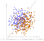
  • \(\sigma(x^{\top} \beta) > 1/2\) exactly when \(x^{\top} \beta > 0\), so the boundary \(\{x : x^{\top} \beta = 0\}\) is a hyperplane
  • Nonlinear boundaries come from nonlinear features (polynomials, interactions, embeddings), as in least squares
  • Points near the boundary have \(p \approx 1/2\): that is where the mistakes are
Decision Rules and Evaluation

The Confusion Matrix

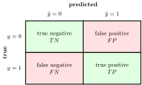
  • Cross-tabulate the true class against the predicted class on data the classifier did not see
  • Rows are the truth, columns the prediction (the sklearn convention)
  • Two kinds of mistakes with different costs: a false positive (predicted \(1\), truly \(0\)) and a false negative (predicted \(0\), truly \(1\))
  • The same matrix returns for k-means next lecture, where cluster labels are arbitrary
Accuracy, Precision, and Recall

  • Accuracy \((TP + TN) / N\); precision \(TP / (TP + FP)\), how much to trust a predicted \(1\); recall \(TP / (TP + FN)\), how many true \(1\)s were found
  • The false positive rate \(FP / (FP + TN)\) and the false negative rate \(1 - \text{recall}\) are what the measurement-error results at the end use
y_hat = clf.predict(X)
print(confusion_matrix(y, y_hat))
print(f"accuracy {clf.score(X, y):.3f}, precision "
      f"{precision_score(y, y_hat):.3f}, recall {recall_score(y, y_hat):.3f}")
[[158  67]
 [ 57 218]]
accuracy 0.752, precision 0.765, recall 0.793

Rare Classes Break Accuracy

  • With \(3\%\) positives, always predicting \(0\) is \(97\%\) accurate and useless
p_rare = expit(-4.0 + X @ beta_true)
y_rare = (rng.random(N) < p_rare).astype(int)
clf_rare = LogisticRegression(C=np.inf).fit(X, y_rare)
y_hat_rare = clf_rare.predict(X)
print(f"share y = 1: {y_rare.mean():.3f}, always-zero accuracy: "
      f"{1 - y_rare.mean():.3f}, classifier accuracy: {clf_rare.score(X, y_rare):.3f}")
print(confusion_matrix(y_rare, y_hat_rare))
print(f"recall {recall_score(y_rare, y_hat_rare):.3f}")
share y = 1: 0.048, always-zero accuracy: 0.952, classifier accuracy: 0.950
[[473   3]
 [ 22   2]]
recall 0.083
  • Report precision and recall whenever a class is rare, which is most variables economists want to code: a strike, a discrimination complaint, a recession

The Threshold is a Cost Decision

  • predict uses \(\hat{y} = \mathbf{1}\left\{{\hat{p}(x) > 1/2}\right\}\). With a false positive costing \(c_{FP}\) and a false negative \(c_{FN}\), the cheaper prediction is \(\hat{y} = 1\) when

\[ \hat{p}(x) > \frac{c_{FP}}{c_{FP} + c_{FN}} \equiv \tau \]

  • Equal costs give \(\tau = 1/2\); if a miss is nine times worse than a false alarm, \(\tau = 0.1\)
  • \(\hat{p}(x)\) estimates the posterior \(\mathbb{P}(y = 1 \,|\, x)\) of the probability lecture. Logistic regression models it directly; generative classifiers such as naive Bayes model \(\mathbb{P}(x \,|\, y)\) and \(\mathbb{P}(y)\) and use Bayes’ law
  • Lowering \(\tau\) raises recall at the expense of false alarms; class_weight="balanced" pushes the fit the same way

The ROC Curve

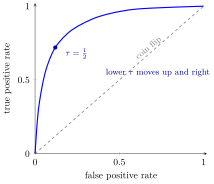
  • Sweep \(\tau\) from \(1\) to \(0\) and plot recall against the false positive rate: the receiver operating characteristic. \(\tau = 1\) flags nothing, \(\tau = 0\) flags everything, a coin flip traces the diagonal
  • Every point is a threshold you could choose: the whole recall-versus-false-alarm menu, before any cost is decided
  • The area under the curve (AUC) is the probability that a random true \(1\) scores above a random true \(0\): a grade for the ranking, independent of \(\tau\)
ROC in Code: the Rare Class Ranks Fine

  • RocCurveDisplay draws the sweep from predict_proba; roc_auc_score integrates it
fig, ax = plt.subplots(figsize=(4.5, 3.4))
s_bal = clf.predict_proba(X)[:, 1]
s_rare = clf_rare.predict_proba(X)[:, 1]
RocCurveDisplay.from_predictions(
    y, s_bal, ax=ax, name="balanced")
RocCurveDisplay.from_predictions(
    y_rare, s_rare, ax=ax, name="rare class")
plt.show()
for tau in [0.5, 0.1]:
    y_hat = (s_rare > tau).astype(int)
    print(f"tau = {tau}: recall "
          f"{recall_score(y_rare, y_hat):.2f}")
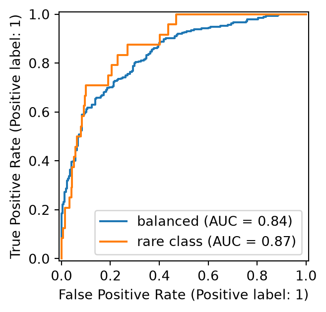
tau = 0.5: recall 0.08
tau = 0.1: recall 0.71
  • The rare-class classifier has the higher AUC: it ranks the positives well and only the default threshold was wrong; at \(\tau = 0.1\) it finds most of them. For a rare class the precision-recall curve (PrecisionRecallDisplay) is the more demanding picture

Train, Test, and Overfitting

  • Fit on a training set, evaluate on a test set the fit never touched. Tune anything (C, the threshold, the features) on a separate validation set, or the test set stops being one
  • Add \(200\) noise features: the MLE fits the training half perfectly and the test half badly
X_noise = np.hstack([X, rng.normal(size=(N, 200))])
X_tr, X_te, y_tr, y_te = train_test_split(X_noise, y, test_size=0.5,
                                          random_state=526)
mle = LogisticRegression(C=np.inf, max_iter=5000).fit(X_tr, y_tr)
lasso = LogisticRegression(l1_ratio=1.0, solver="liblinear", C=0.1).fit(X_tr, y_tr)
oracle = LogisticRegression(C=np.inf).fit(X_tr[:, :2], y_tr)
print(f"MLE:    train {mle.score(X_tr, y_tr):.3f}  test {mle.score(X_te, y_te):.3f}")
print(f"lasso:  train {lasso.score(X_tr, y_tr):.3f}  test {lasso.score(X_te, y_te):.3f}"
      f"  nonzero {(lasso.coef_ != 0).sum()} of {X_noise.shape[1]}")
print(f"oracle: test {oracle.score(X_te[:, :2], y_te):.3f} (the two true features)")
MLE:    train 1.000  test 0.640
lasso:  train 0.788  test 0.736  nonzero 19 of 202
oracle: test 0.740 (the two true features)
  • The lasso drops most of the noise features and nearly matches the model that knows which two matter

More Than Two Classes

Multinomial Logit, the Softmax, and Random Utility

  • With \(K\) classes, give each its own \(\beta_k \in {\mathbb{R}}^M\) and apply the softmax

\[ \mathbb{P}(y = k \,|\, x) = \frac{e^{x^{\top} \beta_k}}{\sum_{j=1}^K e^{x^{\top} \beta_j}} \]

  • Only differences \(\beta_k - \beta_j\) matter, so one class is normalized to \(\beta_1 = 0\); with \(K = 2\) this is the sigmoid. The log-likelihood is still concave, and LogisticRegression fits it automatically when y has more than two values
  • Economists reached the same formula through discrete choice (McFadden 1974): an agent picks the option with the highest utility \(U_k = x^{\top} \beta_k + \epsilon_k\) with i.i.d. Gumbel \(\epsilon_k\), and \(\mathbb{P}(\text{choose } k \,|\, x)\) is the softmax
  • The same map from a score per option to a distribution is how a language model picks the next token, with \(K\) the vocabulary size

Application: Coding Occupations from Job Titles

The Problem

  • Payroll files, postings, and surveys carry free-text titles: POLICE OFFICER, SR DATA ANALYST, Chief Diversity Officer (CDO). Analysis wants a Standard Occupational Classification (SOC) code, whose first two digits give one of \(23\) major groups
  • Hand-coding is slow and inconsistent, so code a labelled sample and classify the rest. O*NET publishes \(8{,}189\) worker-reported titles with their SOC code

Bag of Words

  • The simplest feature map counts how often each vocabulary word appears, ignoring order. CountVectorizer builds the vocabulary from the training titles and returns a sparse matrix with one column per word
demo = CountVectorizer().fit(["Police Officer", "Police Sergeant", "Chief Officer"])
print(demo.get_feature_names_out())
print(demo.transform(["Police Officer", "Police Sergeant"]).toarray())
['chief' 'officer' 'police' 'sergeant']
[[0 1 1 0]
 [0 0 1 1]]
  • Words never seen in training are dropped at prediction time. The text lecture adds weighting and embeddings; counting is enough here

Loading the Data

  • The data files live in slides/data/ of the course repository. The notebooks read a local copy if there is one and the course website otherwise
def data_path(name):
    url = "https://jlperla.github.io/grad_econ_datascience/slides/data/"
    return f"data/{name}" if os.path.exists(f"data/{name}") else url + name

onet = pd.read_csv(data_path("onet_titles.csv.gz"))
sample = onet.sample(4, random_state=1)[["title", "soc_code", "major_group_title"]]
print(sample.to_string(index=False))
print(onet["major_group_title"].value_counts().head(4))
                                      title   soc_code                      major_group_title
              MHA (Mental Health Assistant) 29-2053.00 Healthcare Practitioners and Technical
                            Line Supervisor 51-1011.00                             Production
Home Care Physical Therapist (Home Care PT) 29-1123.00 Healthcare Practitioners and Technical
                  Licensed Reactor Operator 51-8011.00                             Production
major_group_title
Production                                1016
Healthcare Practitioners and Technical     734
Educational Instruction and Library        613
Construction and Extraction                534
Name: count, dtype: int64

Fitting the Coder

  • Word counts of the title, the major group as the label (\(22\) classes), a quarter of the titles held out
vec = CountVectorizer()
X_onet = vec.fit_transform(onet["title"])
y_onet = onet["major_group_title"]
X_tr, X_te, y_tr, y_te = train_test_split(X_onet, y_onet, test_size=0.25,
                                          random_state=526)
coder = LogisticRegression(solver="newton-cg").fit(X_tr, y_tr)
print(f"vocabulary size {X_onet.shape[1]}, classes {len(coder.classes_)}")
print(f"train accuracy {coder.score(X_tr, y_tr):.3f}, "
      f"test accuracy {coder.score(X_te, y_te):.3f}")
vocabulary size 3355, classes 22
train accuracy 0.861, test accuracy 0.719
  • newton-cg is the Newton iteration from earlier; the default solver is ten times slower here. Train well above test: overfitting again

Where Does it Go Wrong?

top = y_onet.value_counts().index[:6]
ConfusionMatrixDisplay.from_predictions(
    y_te, coder.predict(X_te), labels=top,
    display_labels=[t[:22] for t in top],
    xticks_rotation=40, colorbar=False)
plt.tight_layout()
plt.show()

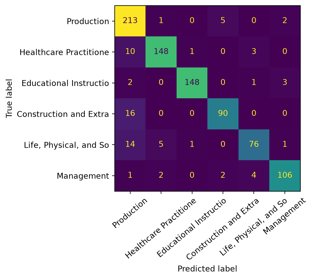
  • The six largest groups on held-out titles. The off-diagonal mistakes are between groups whose titles share words

Coding a Payroll File

  • Apply the coder to \(8{,}000\) full-time salaried positions from the City of Chicago’s payroll
chicago = pd.read_csv(data_path("chicago_payroll.csv.gz"))
X_chicago = vec.transform(chicago["job_title"])
chicago["group"] = coder.predict(X_chicago)
chicago["p_max"] = coder.predict_proba(X_chicago).max(axis=1).round(2)
counts = chicago.groupby(["job_title", "group"])["p_max"].agg(n="size", p_max="first")
print(counts.sort_values("n", ascending=False).head(8).to_string())
                                                                                  n  p_max
job_title                              group                                              
POLICE OFFICER                         Protective Service                      2465   0.89
FIREFIGHTER-EMT                        Healthcare Practitioners and Technical   550   0.18
SERGEANT                               Production                               447   0.15
POLICE OFFICER (ASSIGNED AS DETECTIVE) Protective Service                       376   0.99
FIREFIGHTER-EMT (RECRUIT)              Healthcare Practitioners and Technical   171   0.18
LIEUTENANT-EMT                         Protective Service                       144   0.13
FIRE ENGINEER-EMT                      Architecture and Engineering             141   0.75
PARAMEDIC                              Healthcare Practitioners and Technical   132   0.22
  • Chicago’s titles use a different dialect: FIREFIGHTER-EMT is coded by its second word, and a title with no known word gets the largest-intercept group. Check the common titles and p_max before using the codes

The Regression the Codes Were Built For

premia = smf.ols("np.log(annual_salary) ~ C(group) + C(department)",
                 data=chicago).fit()
coef = premia.params.filter(like="group").round(2)
coef.index = coef.index.str.replace(r"C\(group\)\[T\.(.*)\]", r"\1", regex=True)
print(pd.concat([coef.nsmallest(4), coef.nlargest(4)]).to_string())
Building and Grounds Cleaning and Maintenance   -0.38
Healthcare Support                              -0.29
Healthcare Practitioners and Technical          -0.20
Office and Administrative Support               -0.18
Personal Care and Service                        0.26
Educational Instruction and Library              0.19
Management                                       0.19
Production                                       0.19
  • Log-salary differences relative to Architecture and Engineering within a department, the four lowest and four highest
  • Plausible magnitudes, but the regressor is a classifier’s output with about \(25\%\) of titles miscoded on held-out data: measurement error in a regressor. What does it do to the coefficients?

Generated Regressors

A Coded Regressor is Mismeasured (Aigner 1973)

  • The true \(d_n \in \{0, 1\}\) enters \(y_n = \alpha + \beta\, d_n + u_n\), but we observe the classifier’s \(\hat{d}_n\), with the error rates of its confusion matrix

\[ p_0 \equiv \mathbb{P}(\hat{d}_n = 1 \,|\, d_n = 0), \qquad p_1 \equiv \mathbb{P}(\hat{d}_n = 0 \,|\, d_n = 1) \]

  • If the mistakes are non-differential (given \(d_n\), independent of \(u_n\) and the other regressors), OLS on \(\hat{d}_n\) converges to

\[ \hat{\beta} \approx \beta \cdot \lambda, \qquad \lambda \approx 1 - p_0 - p_1 \]

  • For any classifier better than a coin flip (\(p_0 + p_1 < 1\)), \(\lambda\) is between \(0\) and \(1\): attenuation toward zero, never a sign flip, unchanged as \(N\) grows

Monte Carlo

def attenuation(N, p0, p1, pi=0.3, beta=1.0, reps=100):
    slopes = []
    for _ in range(reps):
        d = rng.random(N) < pi
        y = 2.0 + beta * d + rng.normal(size=N)
        d_hat = np.where(d, rng.random(N) > p1, rng.random(N) < p0).astype(float)
        slopes.append(sm.OLS(y, sm.add_constant(d_hat)).fit().params[1])
    return np.mean(slopes)

for N in [1_000, 10_000, 100_000]:
    print(f"N = {N:>7,}: mean slope {attenuation(N, 0.05, 0.20):.3f}")
pi, q = 0.3, 0.3 * 0.8 + 0.7 * 0.05
print(f"1 - p0 - p1 = {0.75:.3f}, exact factor {0.75 * pi * (1 - pi) / (q * (1 - q)):.3f}")
N =   1,000: mean slope 0.789
N =  10,000: mean slope 0.789
N = 100,000: mean slope 0.789
1 - p0 - p1 = 0.750, exact factor 0.790
  • True \(\beta = 1\). The estimate sits at the exact factor \((1 - p_0 - p_1)\, \pi(1 - \pi) / (q(1 - q))\), with \(q\) the predicted share of ones, and does not move with \(N\)

Corrections Exist

  • The held-out confusion matrix estimates \(p_0\) and \(p_1\), so the attenuation can be undone. Three to know about
    • Battaglia, Christensen, Hansen, and Sacher (2024): correct the moments with the validation-sample error rates; package ValidMLInference
    • Prediction-powered inference (Angelopoulos et al. 2023): combine predictions on the full sample with the labelled sample into an unbiased estimator
    • Design-based supervised learning (Egami, Hinck, Stewart, and Wei 2023): the same idea for text, with the labelled sample drawn at random from the corpus
  • The common thread: keep a random labelled sample, never treat classifier output as truth, and report the confusion matrix with the regression. The text lecture applies the same factor to a misclassified outcome