Rethinking Least Squares: Min-Norm Solutions and Loss Geometry
Machine Learning Fundamentals for Economists
Overview
Motivation
- In preparation for the ML lectures we cover some core numerical linear algebra concepts on functional equations
- We will also use this as an opportunity to reinterpret least squares solutions as a prelude to non-linearity
- Connection to previous lecture: conditioning and eigenvalues drive algorithm behavior
Why This Matters for ML
- Modern ML operates in high-dimensional parameter spaces where traditional “identification” fails
- Neural networks: millions of parameters, infinitely many equivalent solutions
- Yet these models generalize well despite apparent non-uniqueness
- Key insight: multiplicity of parameters \(\neq\) multiplicity of the functions they represent
- Different \(\beta\) may produce the same (or nearly same) predictions
- Understanding this requires thinking about geometry of loss functions
- This lecture builds intuition through the simplest case: linear least squares
- Same geometric principles extend to deep learning
Packages and Materials
Least Squares with the QR Decomposition
Least Squares and Normal Equations
- Given the least squares problem
\[ \min_x \| Ax -b \|^2 \]
- Taking the FOCs and rearranging gives the normal equations
\[ A^\top A x = A^\top b \quad \Rightarrow \quad x = (A^\top A)^{-1} A^\top b \]
- This works, but forming \(A^\top A\) can be numerically unstable
- Condition number squares: \(\kappa(A^\top A) = \kappa(A)^2\)
QR Decomposition for Least Squares
- QR factorizes rectangular matrices: \(A = Q R\) for \(Q\) orthogonal, \(R\) upper triangular
- Substitute \(A = QR\) into the normal equations \(A^\top A x = A^\top b\):
\[ (QR)^\top (QR) x = (QR)^\top b \]
\[ R^\top Q^\top Q R x = R^\top Q^\top b \]
- Since \(Q^\top Q = I\) (orthogonal), this simplifies to \(R^\top R x = R^\top Q^\top b\)
- Left-multiply by \((R^\top)^{-1}\) to get the triangular system:
\[ R x = Q^\top b \]
- Solve via back-substitution - avoids forming \(A^\top A\) entirely, much more stable
QR is Used Internally for Least Squares
- Inside
lstsqand similar functions, QR is used for numerical stability - Compare direct normal equations vs. QR-based solution
N, M = 10, 3
A = np.random.randn(N, M) + np.random.randn(N, 1)
b = np.random.randn(N)

# QR-based solution
x_lstsq, residuals, rank, s = lstsq(A, b)

# Normal equations (less stable but instructive)
x_normal = solve(A.T @ A, A.T @ b)
print(f"lstsq solution: {x_lstsq}")
print(f"Normal eqn sol: {x_normal}")
lstsq solution: [-0.4229563 0.63714154 -0.16902314]
Normal eqn sol: [-0.4229563 0.63714154 -0.16902314]QR and Underdetermined Least Squares
- Take the case where \(N < M\) and use the QR decomposition
Solution: [-3.05555556  0.11111111  3.27777778]
Rank: 2, Columns: 3- Wait, why did that give an answer?
- And if I try various algorithms even with random starting points, why does it give the same answer?
- There is a bias towards a particular solution. Will come back to this repeatedly
Min-Norm Solutions and Sobolev Spaces
Min-Norm Solution
- Linear least squares was solving \(\min_x \| Ax -b \|_2^2\)
- Which had multiplicity in this case. The solution it returns fulfills
\[ \min_x \| x \|_2^2 \quad \text{s.t.} Ax = b \]
- Or, can think of as solving the “ridgeless regression”
\[ \lim_{\lambda \to 0}\left[\min_x \| Ax -b \|_2^2 + \lambda \| x \|_2^2\right] \]
- Will become crucial in deep learning where the number of parameters \(\gg\) data
Algorithms + Optimization Problems
- A key requirement to make the switch to ML thinking is to remember that just seeing the optimization problem, e.g. \(\max_{x} f(x)\) may not be enough
- The algorithm itself will be important if there is multiplicity in solutions, if things are not numerically stable, etc.
- In the case above, we saw that using QR decomposition delivered the min norm
Linear Operators, not Matrices
- Recall: for \(x \in {\mathbb{R}}^N\) we should think of \(f(x) = A x\) for \(A\in{\mathbb{R}}^{M \times N}\) as a linear transformation from \({\mathbb{R}}^N\) to \({\mathbb{R}}^M\)
- Definition of Linear: \(f(a x_1 + b x_2) = a f(x_1) + b f(x_2)\) for scalar \(a,b\)
- Many algorithms might be implementable just using the matrix-vector product or the transpose of the matrix-vector product?
- Maybe we don’t actually need to create a matrix? Can compose operations together?
- This will be related to a lot of ML algorithms and autodifferentiation. Hint: Jacobian \(\nabla f(x) = A\)
- The key to iterative methods will be the spectral properties of the Jacobian, which is related to the eigenvalues of \(A\)
\(L^p\) Space
Let \(\Omega\) be an open subset of \({\mathbb{R}}^n\). A function \(u: \Omega \rightarrow {\mathbb{R}}\)
\(L^p(\Omega)\) space: A function \(f: \Omega \rightarrow {\mathbb{R}}\) is in \(L^p(\Omega)\) if:
\[ \int_\Omega |f|^p \, dx < \infty \]
- Useful in a lot of cases, but will be especially important when considering norms on a function space and whether a particular function solves a particular problem
Sobolev Space
A function \(u\) belongs to the Sobolev space \(W^{k,p}(\Omega)\) if:
\[ u \in L^p(\Omega) \]
and all its weak derivatives up to order \(k\) are also in \(L^p(\Omega)\).
A function \(\phi \in W^{k,p}(\Omega)\) is said to be a weak derivative of \(u\) if:
\[ \int_\Omega u D^\alpha \phi \, dx = (-1)^{|\alpha|} \int_\Omega \phi D^\alpha u \, dx \]
for all multi-indices \(\alpha\) with \(|\alpha| \leq k\).
Sobolev Norm
The Sobolev Norm for a function \(u \in W^{k,p}(\Omega)\) is defined as some variation on:
\[ \| u \|_{W^{k,p}(\Omega)} = \left( \sum_{|\alpha| \leq k} \int_\Omega |D^\alpha u|^p \, dx \right)^{1/p} \]
where \(\alpha\) is a multi-index and \(D^\alpha u\) represents the weak derivative of \(u\).
You can choose whatever terms you want in \(\alpha\)
A Key Sobolev Semi-Norm
The key one to keep in mind is \(W^{1,2}(\Omega)\), which is the space of functions with square-integrable first derivatives.
\[ \| u \|_{W^{1,2}(\Omega)} = \left( \int_\Omega |\nabla u|^2 \, dx \right)^{1/2} \]
- Note that we have the option to include or not include the \(|u|^2\) term itself when we define a particular norm
- This is a semi-norm because it is semi-definite (i.e., multiple \(u\) with \(\|u\| = 0\))
- Semi-norms serve two key purposes: establish equivalence classes, and prove a way to control length which will come up with algorithms
Sobolev Semi-Norms and Equivalence Classes
- A Sobolev semi-norms \(S\) define equivalence classes of functions
- i.e., any \(u_1\) and \(u_2\) such that \(\|u_1 - u_2\|_S = 0\) are in the same equivalence class
- In general, when we move to nonlinear and highly parameterized models there will be many solutions that are equivalent
- But if they are in approximately the same equivalence class, then who cares?
- Multiplicity of “parameters” doesn’t really matter if the functions do the same thing
Sobolev Semi-Norms and Occam’s Razor
- The other purpose is to give some sense of length, \(\|u_1\|_S < \|u_2\|_S\)
- This will come up with regularization since we may want to bias algorithms towards particular functions or interpret inherent bias in the algorithms
- The key interpretation here is that for Sobolev Norms we can think of variations on the \(W^{1,2}\) as determining how simple a function is
- If \(\|u_1\|_S < \|u_2\|_S\) then it has smaller gradients and fewer “wiggles”
- If both interpolate the same data, then we should prefer the simpler one. Occam’s Razor
- We won’t always be able to know the precise semi-norm when working with ML, but this is useful intuition
Sobolev Norms and Linear Functions
- Now, think of linear functions \(f(x) = \beta x\) where \(\beta\) is a vector, matrix, or scalar
- Consider this on a bounded domain \(\Omega\) so the integrals are well defined
- Then our Sobolev 1,2 norm, \(W^{k,p}\) here is simple:
\[ \|f\|_{W^{1,2}} = \|\beta\|_2 \]
Where \(\|\beta\|_2\) is euclidean norm of the vector, or the Frobenius norm of the matrix
Back to the Ridgeless Regression
Now lets reinterpret our “ridgeless regression” with a
\[ \lim_{\lambda \to 0}\left[\min_{\beta} \| A\beta -b \|_2^2 + \lambda \| \beta \|_2^2\right] \]
- This says that we are “penalizing” the norm of \(f(x) = \beta x\) in the \(W^{1,2}\) sense
- The limit \(\lambda \to 0\) means we are asymptotically dropping this penalty, but there is still this “bias” which makes solutions unique
- Normally unique to an equivalence class with in \(W^{1,2}\), but with linear functions they are unique. Why?
Min-Norm Solution as Occam’s Razor
Recall that this was also
\[ \min_{\beta} \| \beta \|_2^2 \quad \text{s.t.}\, A\beta = b \]
- i.e., we are finding the minimum norm solution that interpolates our data
- And we can interpret the minimum norm through Occam’s Razor
- This general principle will apply when we think about nonlinear approximations as well, though we don’t need to fully interpolate (i.e., if \(\lambda > 0\) then we don’t need to interpolate perfectly)
- Suggests the crucial role of regularization.
Singular Linear Systems of Equations
This isn’t just least squares
- Consider the case for finding solutions to \(A \beta = b\) where \(A\) is singular.
- Either no solution or infinite solutions exist
- If you solve a linear system with SVD or iterative methods it gives an answer! The min-norm solution
\[ \begin{aligned} \min_{\beta} & \,\| \beta \|_2^2\\ &\text{s.t.} A\beta = b \end{aligned} \]
Is the Min-Norm Solution Special?
The min-norm solution to LLS is the closest projection to the column space of the data
For a given norm it is the unique solution to a well-specified problem which can often be interpreted through appealing to simplicity
It is also the unique “most stable” solution for a given norm. Loosely,
- Take \(b + \delta b\) for some small \(\delta b\) and/or \(A + \delta A\) for some small \(\delta A\)
- Then the min-norm solution is the one where \(\beta + \delta \beta\) is smallest
Another interpretation we will apply to ML and nonlinear models: min-norm solutions are the ones least sensitive to data perturbations
This will also come up with Bayesian statistics, if we apply a prior which is asymptotically non-informative, the min-norm solution is the MAP solution
Min-Norm Solution and Conditioning
- As a preview of connections to the previous lecture, consider if the matrix is almost, but not quite singular
- Tough to know due to numerical roundoff
- You may have learned from experience that everything works great if you:
- Tweak to the diagonal of the matrix, or to the normal equations for LLS, or to make a covariance matrix positive definite
- Consider how that is related to the min-norm solution and L2 penalized LLS (i.e., “ridge”)
- Will turn out to be exactly equivalent in many algorithms
Geometry and Loss Functions
Geometry of Loss Functions
- The curvature of the loss function will be essential to understanding generalization
- The motivation: we will work with models where every local minima is a global minima, multiplicity is pervasive but innocuous, etc.
- For some \(\beta^*\) which is a local minima of \(\min_{\beta} f(X;\beta)\) the Hessian \(\nabla^2 f(X;\beta^*)\) tells us about whether minima are unique, how sensitive they are to perturbations, etc.
- Key questions to ask:
- What is the rank of the hessian? If full rank, with a positive definite hessian, then the solution is (locally) unique
- Eigenvalues show ridges/etc.
Geometry of Regularized LLS
\[ \min_{\beta} \underbrace{\frac{1}{2}\left[\| X\beta -y \|_2^2 + \lambda \| \beta \|_2^2\right]}_{\equiv f(X;\beta)} \]
- The Hessian is then (for all \(\beta\))
\[ \nabla^2 f(X;\beta^*) = X^{\top} X + \lambda I \]
- Is this problem convex with \(\lambda = 0\)? Only if \(X^{\top}X\) is positive definite
Reminder on Positive and Semi-Definite
Positive definite if \(x^{\top} A x > 0,\) (“semi-definite” if \(\geq 0\)) for all \(x \neq 0\)
With the spectral decomposition of symmetric \(A\)
\[ A = Q \Lambda Q^{\top} \]
- \(\Lambda = \text{diag}(\lambda_1, \ldots, \lambda_n)\) and \(Q\) is an orthogonal matrix of eigenvectors
- \(A\) is positive definite if \(\lambda_i > 0\) for all \(i\)
- \(A\) is positive semi-definite if \(\lambda_i \geq 0\) for all \(i\)
In more abstract and infinite dimensional spaces a linear operator \(A(x)\) operator is positive definite if \(x \cdot A(x) > 0\) for all \(x \neq 0\)
- Has eigenvalues/eigenvectors, i.e. \(A(x) = \lambda x\) for some \(\lambda\) and \(x\)
Shape of Positive Definite Function
- For \(A = \begin{bmatrix} 3 & 1 \\ 1 & 2\end{bmatrix}\) (positive definite)
- This has a unique minimum (at \((0, 0)\), since no “affine” term)
Eigenvalues: [1.38196601 3.61803399] (all positive)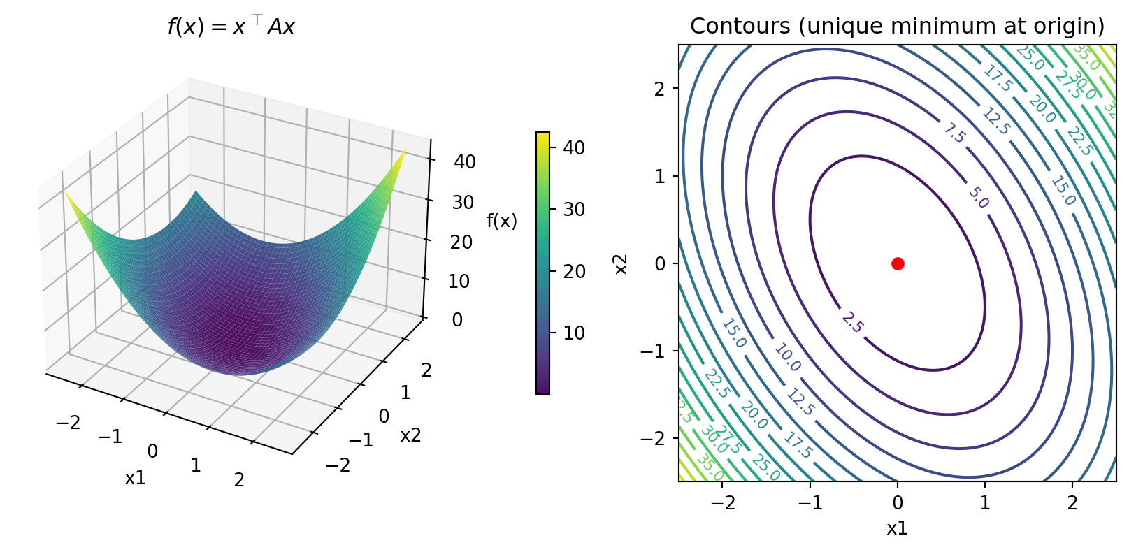
Shape of Positive Semi-Definite Function
- For \(A = \begin{bmatrix} 1 & 1 \\ 1 & 1\end{bmatrix}\) (positive semi-definite, not definite)
- Multiple minima along a line! The zero eigenvalue creates a “ridge”
Eigenvalues: [0. 2.] (one is zero!)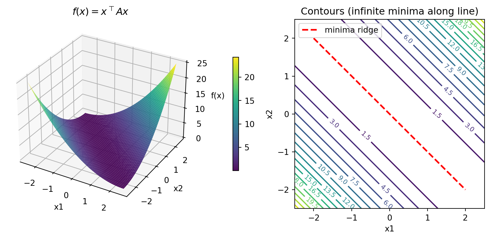
Shape of Indefinite Function (Saddle Point)
- For \(A = \begin{bmatrix} 1 & 0 \\ 0 & -1\end{bmatrix}\) (indefinite: positive and negative eigenvalues)
- No minimum or maximum at origin - it’s a saddle point
Eigenvalues: [-1. 1.] (mixed signs = indefinite)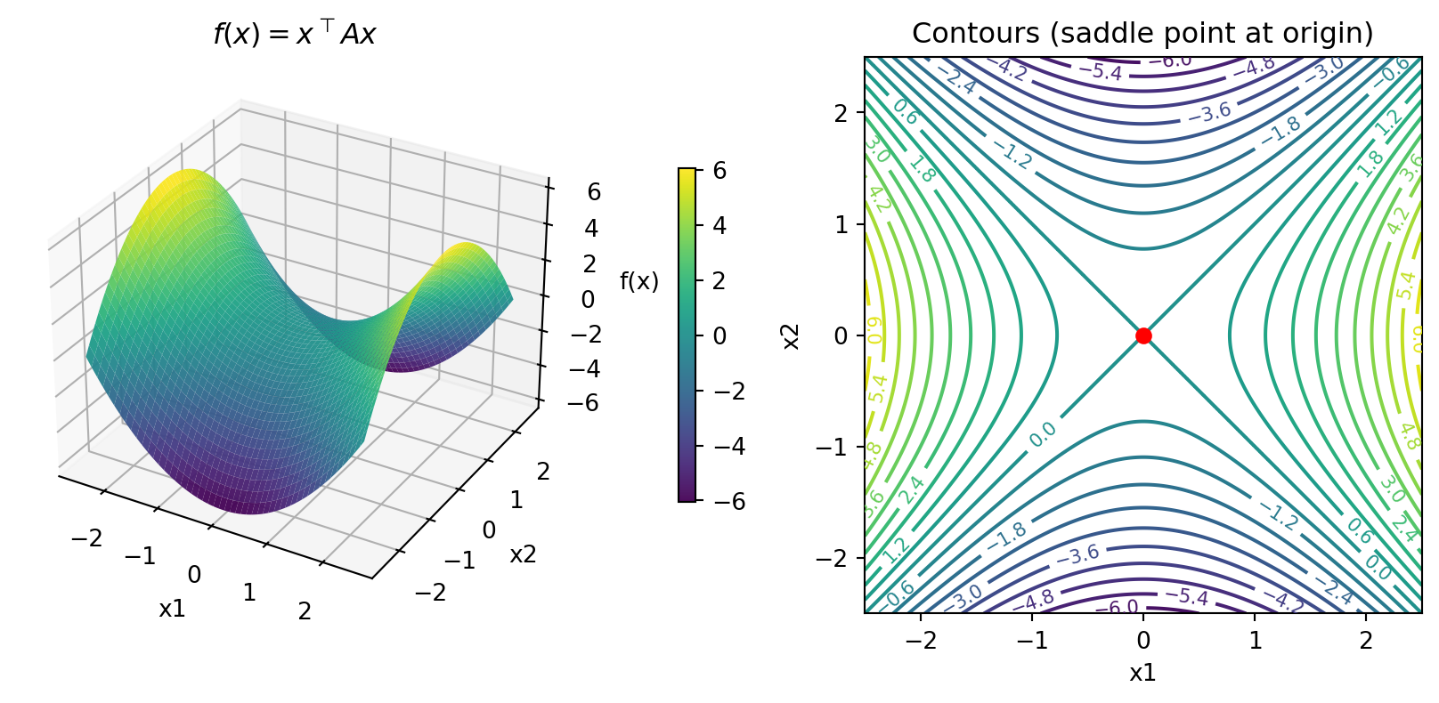
Regularization Creates Unique Minimum
- Take semi-definite \(A = \begin{bmatrix} 1 & 1 \\ 1 & 1\end{bmatrix}\) and add \(\lambda I\) for \(\lambda = 0.1\)
- Now unique minimum at \((0, 0)\)!
Eigenvalues after regularization: [0.1 2.1] (both positive now)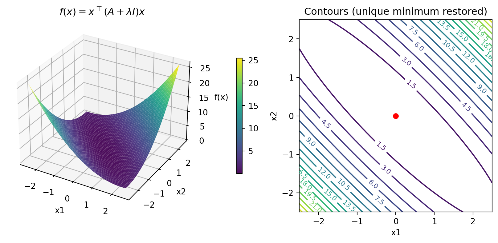
Convexity of a Quadratic Objective
- We will build \(P\) and \(f(x) = \frac{1}{2}x^{\top} P x\) from the spectral decomposition
- Rotating eigenvectors and starting with \(\Lambda = \text{diag}(1, 1)\)
- And keep in mind that \(\nabla f(x) = P x\)
Contours of the Quadratic Objective
x_vals = np.linspace(-1, 1, 100)
X1, X2 = np.meshgrid(x_vals, x_vals)
Z = 0.5 * (P[0,0]*X1**2 + 2*P[0,1]*X1*X2 + P[1,1]*X2**2)
plt.figure(figsize=(6, 5))
cs = plt.contour(X1, X2, Z, levels=20, cmap='viridis')
plt.clabel(cs, inline=True, fontsize=8)
plt.xlabel('x1'); plt.ylabel('x2')
plt.title(r'$f(x) = \frac{1}{2} x^\top P x$ with $\Lambda = (1, 1)$')
plt.gca().set_aspect('equal')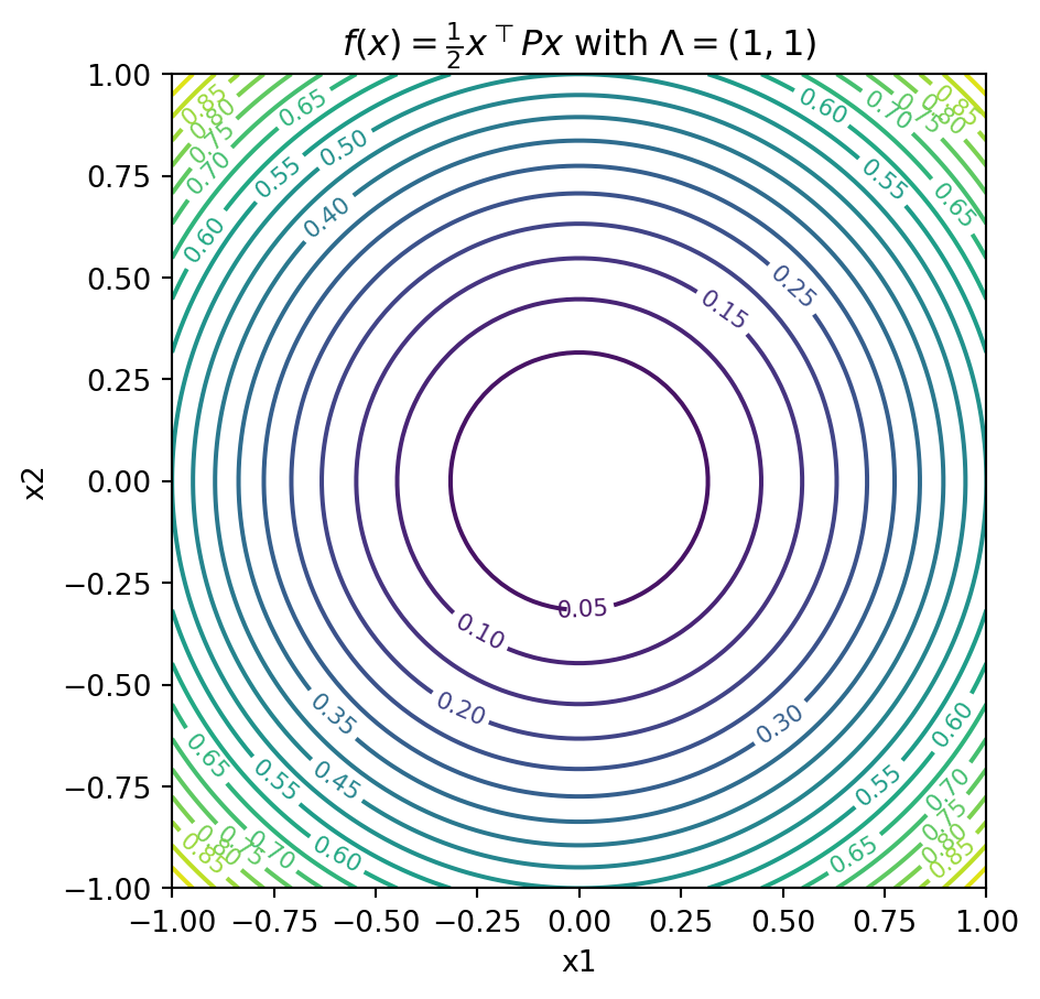
Gradient Descent and Conditioning
Gradient Descent Style Algorithms
- To understand the importance of geometry, lets consider optimizing with simple gradient descent style algorithms to minimize:
\[ \min_{x} \frac{1}{2}x^{\top} P x \]
- Let \(\eta > 0\) be a “step size”, learning rate, etc. then
\[ x^{i+1} = x^i - \eta \nabla f(x^i) = x^i - \eta P x^i \]
- We will fix \(x^0 \equiv \begin{bmatrix}0.9 & 0.0\end{bmatrix}\), set \(\eta = 0.5\) and plot a few iterations
Gradient Descent Visualization Code
def plot_gd_steps(N_steps, x_0, Lambda, eta):
    Q = np.array([[np.sqrt(2)/2, np.sqrt(2)/2],
                  [-np.sqrt(2)/2, np.sqrt(2)/2]])
    P = Q @ np.diag(Lambda) @ Q.T
    gd_step = lambda x: x - eta * P @ x
    x_vals = np.linspace(-1, 1, 100)
    X1, X2 = np.meshgrid(x_vals, x_vals)
    Z = 0.5 * (P[0,0]*X1**2 + 2*P[0,1]*X1*X2 + P[1,1]*X2**2)
    plt.figure(figsize=(6, 5))
    plt.contour(X1, X2, Z, levels=20, cmap='viridis')

    x_current = np.array(x_0)
    for i in range(N_steps):
        x_next = gd_step(x_current)
        plt.arrow(x_current[0], x_current[1], x_next[0] - x_current[0],
        x_next[1] - x_current[1],head_width=0.03, head_length=0.02, fc='red', ec='red')
        x_current = x_next

    plt.xlabel('x1'); plt.ylabel('x2')
    plt.gca().set_aspect('equal')
    return plt.gcf()
Contours With Well-Conditioned Matrices
- Let \(\Lambda = \text{diag}(1, 1)\) which leads to \(P = I\)
- Converges almost immediately. Immediately in any dimensions with \(\eta = 1\)
Contours With Well-Conditioned Matrices
Text(0.5, 1.0, '$\\Lambda = (1, 1)$: Well-conditioned')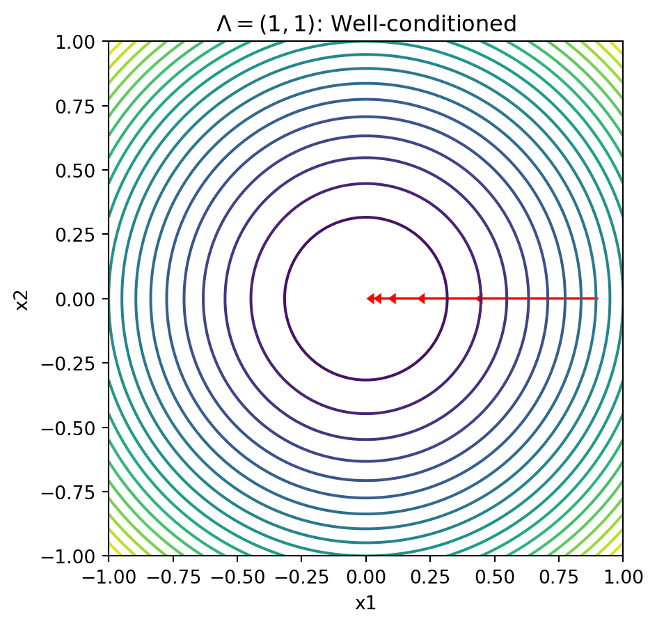
Contours With Less Well-Conditioned Matrices
- Let \(\Lambda = \text{diag}(1, 0.5)\)
- Does great in one direction, but slows down
Contours With Less Well-Conditioned Matrices
Text(0.5, 1.0, '$\\Lambda = (1, 0.5)$: Moderately conditioned')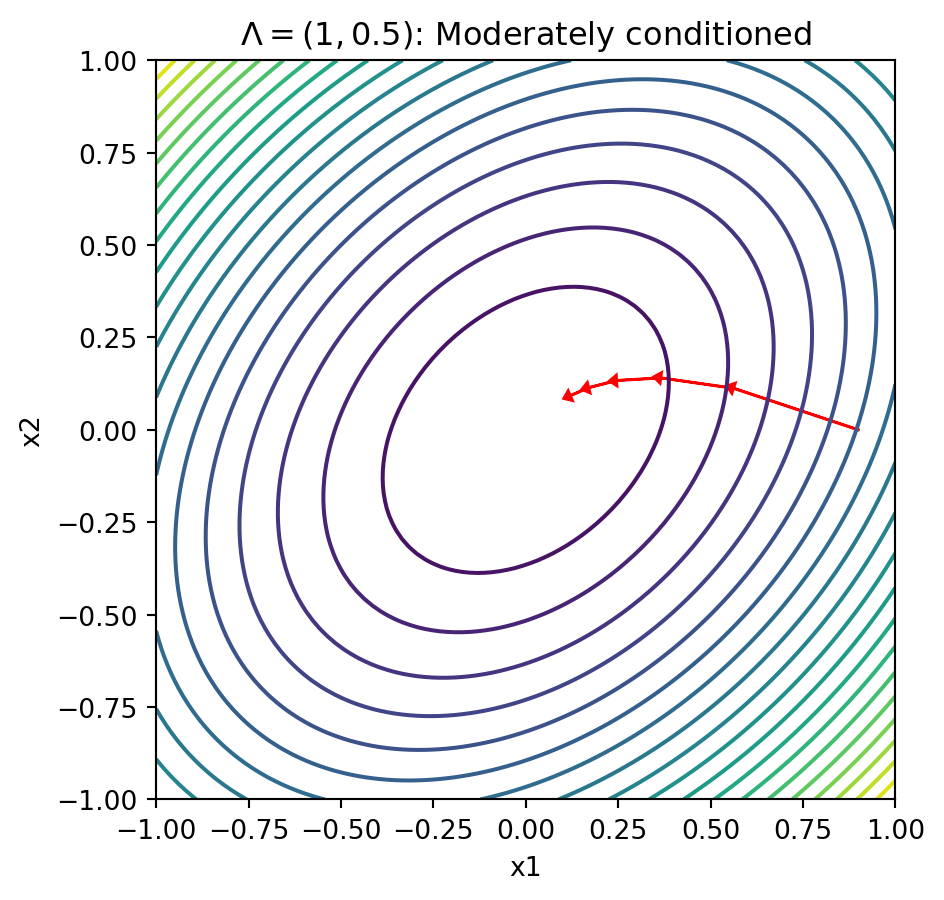
Contours Getting Closer to a “Ridge”
- Let \(\Lambda = \text{diag}(1, 0.1)\)
- Slow convergence in the “flat” direction
Contours Getting Closer to a “Ridge”
Text(0.5, 1.0, '$\\Lambda = (1, 0.1)$: Poorly conditioned')
Contours With Terribly Conditioned Matrices
- Let \(\Lambda = \text{diag}(1, 0.01)\)
- Can barely move in the “bad” direction
Contours With Terribly Conditioned Matrices
Text(0.5, 1.0, '$\\Lambda = (1, 0.01)$: Terribly conditioned')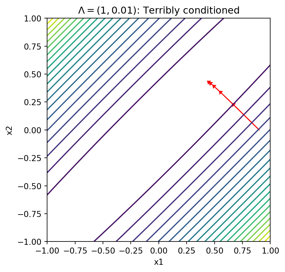
Contours With Ill-Conditioned Matrices
- Let \(\Lambda = \text{diag}(1, 0.0)\)
- Not full rank, positive semi-definite. But hits minima along the ridge
Contours With Ill-Conditioned Matrices
Text(0.5, 1.0, '$\\Lambda = (1, 0)$: Singular (semi-definite)')
Regularization and Large-Scale Methods
Motivation for Regularization and Conditioning
Geometry, not dimensionality, the key to understanding a large class of algorithms (anything you would use in high-dimensions)
- “Local” geometry is summarized by the “spectrum” of the Hessian
- In particular, wildly mismatched eigenvalues are the enemy
\[ \text{cond}(A) = \left|\frac{\lambda_{\max}(A)}{\lambda_{\min}(A)}\right| \]
Regularization: ridge \(\alpha \|x\|_2^2\) then spectrum becomes \(\lambda_i + \alpha\)
See more in Mark Schmidt’s Notes on Gradient Descent
Condition Number and Numerical Precision
- Rule of thumb: if condition number is \(10^k\), lose about \(k\) digits of precision
cond(X) = 1.34
cond(X.T @ X) = 1.80
cond(X_col.T @ X_col) = 1.65e+16
Ridge Regression Stabilizes Conditioning
Iterative Methods for Large-Scale Least Squares
- For very large systems, direct methods become impractical
- The iterative methods lecture covers NormalCG and other Krylov methods
- Lineax
lx.NormalCG()solver for least squares via iterative methods - Key insight: same conditioning/eigenvalue concepts determine convergence rate
- Preconditioners transform the problem to improve conditioning