Introduction to Kernel Methods and Gaussian Processes

Machine Learning Fundamentals for Economists

Jesse Perla

jesse.perla@ubc.ca

University of British Columbia

Overview

Motivation

We have discussed various forms of representation learning and function approximation including neural networks, LLS, etc.
Another type of approach is called “Instance (or Exemplar) Based Learning” of which Kernel Methods and Gaussian Processes are a special case
- The idea there is that we find approximations from the data by keeping track of all observations and use them for inference
- These methods are non-parametric in the sense that the number of parameters grows with the number of data points
- Often Bayesian in practice, which provides regularization and inference

Limitations and Advantages

While it seems like this is limiting to cases with small amounts of data
- We have already explored high-dimensional linear algebra methods (e.g., matrix-free, iterative methods, preconditioning)
- Many problems in economics do not have an enormous number of observations, or we have choice on where the observations occur
Typically these methods are used without any “representation learning”, but at the end we will give some pointers to how these methods generalize to allow representation learning
One major benefit of these methods to economists is that they will provide posteriors in a function space, which we can use for inference

References

These notes are a bare-bones introduction. Look to other references
ProbML Book 1 Section 17 and ProbML Book 2 Section 18
Gaussian Processes for Machine Learning a beloved textbook available online
UBC CPSC 340 and Mark Schmidt’s Topics Notes
Machine Learning with Kernel Methods course with youtube lectures

Normal Equations

Reminder: Normal Equations for Ridge Regression

Let \(x \in \mathbb{R}^M\) be observations and \(X \in \mathbb{R}^{N \times M}\) be the “design” matrix
To solve \(\min_{\theta}\left\{||X \theta - y||^2 + \lambda||\theta||^2\right\}\) for \(\lambda \geq 0\), form normal eqs.

\[ \theta = (X^{\top}X + \lambda I)^{-1} X^{\top} y \]
- The \(X^{\top}X \in \mathbb{R}^{M\times M}\) is in the “feature” space and of size \(M\)

The “Other” Normal Equations

Without proof, turns out you can rearrange this expression to get the “other” normal equations

\[ \theta = X^{\top} (X X^{\top} + \lambda I)^{-1} y \]
- \(X X^{\top} \in \mathbb{R}^{N\times N}\) is called the Gram matrix
- \([X X^{\top}]_{ij} = x_i \cdot x_j\). i.e., pairwise comparisons of all data
Since \(M \ll N\) typically, often a bigger system to solve
- But note that we have rewritten as pairwise comparisons

Prediction with Kernels

Define \(\mathcal{K}(x,x') \equiv x \cdot x'\), then

\[ K_{ij} \equiv [X X^{\top}]_{ij} = \mathcal{K}(x_i, x_j)\,\text{ for i = 1, ..., N and j = 1, ..., N} \]

Now, assume we received \(P\) new points of data \(\tilde{X}\) and want to predict \(\tilde{y}\)

\[ \tilde{K}_{ij} \equiv \mathcal{K}(\tilde{x}_i, x_j),\,\text{ for i = 1, ..., P and j = 1, ..., N} \]

Finally (see linked derivations), can predict with

\[ \tilde{y} = \tilde{K} (K + \lambda I)^{-1} y \]

Are Working with Pairwise Comparisons Better?

We have rewritten the normal equations in terms of pairwise comparisons (the Gram matrix) using some function \(\mathcal{K}(x,x')\equiv x \cdot x'\)
Is this computationally preferable for standard applications of OLS?
- Probably not unless \(M\) is very large
The real advantage is that by rewriting the problem in terms of pairwise comparisons we can generalize to other functions \(\mathcal{K}(x,x')\)
- This is the basis of kernel methods and Gaussian processes

Features and The Kernel Trick

Motivation from Classification

One starting point here is to consider simple problems of separating hyperplanes and binary classification
If we transform our data, sometimes into higher dimensions, then we can find separating hyperplanes
- i.e., with the right “features”, many problems become linear
See CPSC 340

Transforming with Polynomials

https://members.cbio.mines-paristech.fr/~jvert/svn/kernelcourse/slides/master2017/master2017.pdf

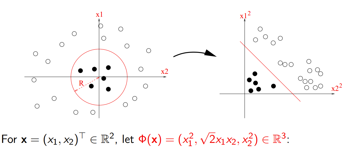
Do we Need to Form the Features?

In the previous with \(x \in \mathcal{D}\), we could have:
- For all \(x\equiv \begin{bmatrix}x_1 & x_2\end{bmatrix}^{\top}\)
- Calculate \(x \mapsto \phi(x) \equiv \begin{bmatrix}x_1^2 & \sqrt{2} x_1 x_2 & x_2^2\end{bmatrix}^{\top}\)
- This is creating our new “features”
- Then run standard classification algorithms on the new features
Define \(\mathcal{K}(x,x') \equiv \phi(x) \cdot \phi(x')\)
- Then use \(\mathcal{K}(x,x')\) rather than explicitly designing the \(\phi(\cdot)\) or calculating \(\phi(x)\) for \(x\in \mathcal{D}\)

Example with Polynomial Kernels

Generalizing our previous case, \(\mathcal{K}(x,x') \equiv (x \cdot x')^2\), to polynomial order \(p\) with cross-products \[ \mathcal{K}(x,x') \equiv (x \cdot x' + c)^p \]
The dimensionality of the underlying \(\phi(x)\) is combinatorial in \(p\)
But now we can just evaluate pairwise \(\mathcal{K}(x,x')\), just an inner product in \(M\) independent of \(p\)!
The cost will be that we need to store the \(N \times N\) matrix of pairwise comparisons

The Kernel Trick

Note in the previous examples that we never formed the \([\phi(x_i)]_{i=1}^N\)
Even further, we didn’t need to even write down the \(\phi(x)\) function explicitly
This is called the “Kernel Trick” and is the basis of Kernel Methods
- By choosing a \(\mathcal{K}(x,x')\) and using “the other normal equations” or similar formulations in other algorithms, you implicitly define features \(\phi(x)\)
- In fact, the \(\phi(x)\) may be infinite dimensional!
The downside is that this will require keeping track of all previous observations (as we did with the normal equations forming \(\tilde{K}\))

Kernelized Methods

Many ML methods are “kernelized”, which means that they are written in terms of pairwise comparisons for a given kernel
- A kernelized regression just takes the standard \(\mathcal{K}(x,x') = x \cdot x'\) and lets us swap out with other \(\mathcal{K}(x,x')\)
For example, the Support Vector Machines (SVM) are just kernelized linear classifiers. There kernelized versions of PCA, etc.
These are powerful because they enable us to work with (often linear) methods in a richer feature space
- But we have to choose the right sorts of kernels to deliver those features
Next we build a little intuition on kernels before formalizing GPs

Kernels

Kernels as Similarity Measures

Our canonical example is \(\mathcal{K}(x,x') = x \cdot x'\), which is a measure of similarity between \(x\) and \(x'\). Note that \[ ||x - x'||_2 = \sqrt{\mathcal{K}(x, x) - 2 \mathcal{K}(x,x') + \mathcal{K}(x', x')} \]
Fix the lengths \(||x||_2 = ||x'||_2 = 1\) then notice that \(||x - x'||_2 = \sqrt{2 (1 - \mathcal{K}(x,x'))}\)
As \(\mathcal{K}(x,x')\) increases, the distance between \(x\) and \(x'\) decreases
Also notice that when \(\mathcal{K}(x,x') = 0\) (i.e. orthogonal since \(x \cdot x' = 0\)) we maximize the distance between \(x\) and \(x'\)

Gaussian Kernel

One of the most commonly used kernels is called the radial basis function(RBF) kernel, also known as the Gaussian kernel

\[ \mathcal{K}(x, x';\ell) \equiv \exp(-\frac{||x - x'||_2^2}{2 \ell^2}) \]

Note that this uses the Euclidean norm, but we could use other norms
The \(\ell\) is a scale which determines the distances over which we expect differences to matter
Kernels which are only a function of some distance between \(x\) and \(x'\) (where the location is irrelevant) are called stationary kernels

Example Kernels

See ProbML Book 2 Section 18.2 for more and Mercer’s Theorem - which shows all kernels are associated with an inner product in some orthonormal feature space
Polynomial kernel \(\mathcal{K}(x,x') = (x \cdot x' + c)^p\) for \(p \in \mathbb{N}\) the polynomial order, including \(p=1\) which is just the linear kernel
Other kernels can be richer and depend on the data (e.g., for network, text, image data). Pick your \(\mathcal{K}(x,x')\) to implement similarity measures
Can construct kernels from other kernels (e.g. \(\exp(\mathcal{K}(x,x'))\) is a valid kernel)
Kernel functions could even be neural networks (Deep Kernels)
Kernels typically have parameters (e.g., \(\ell\) in the Gaussian kernel) which must be fit - usually by maximizing the marginal likelihood

Gaussian Processes

Parameter Space vs. Function Space

There are two basic approaches to understanding Gaussian Processes (GPs)
1. The parameter (or weight) space
2. The function space
See the Gaussian Processes for Machine Learning chapter 2 for more details
Given what you have learned about the kernel trick, you can probably understand a lot of the “parameter space” approach yourself.
Read both, but we will focus on the function space - which is its main advantage

Gaussian Processes

A Gaussian processes are random functions where for any finite set of points \(x_1, ..., x_N \in \mathcal{D}\), the marginal distribution \(f(x_1), ..., f(x_N)\) is a multivariate Gaussian distribution
Another way to think about a GP is that it is a collection of random variables, any finite number of which have a joint Gaussian

Why Random Functions?

The random functions with GPs enable us to have
- distributions over functions
- priors and posteriors in function spaces
- meaningful notions of norms to compare functions and regularize them
Uncertainty Quantification: An issue with ERM-methods (including deep learning) is that they find a single function (think MLE or MAP solutions)
- Alternatives like sample-splitting, cross-validation are limited in their ability to quantify uncertainty
Surrogates: GPs can be used to form probabilistic surrogate functions given data. Then we can use those surrogates for optimization, uncertainty quantification, etc.

Bayesian Optimization and Its Generalizations

One particularly useful application is Bayesian optimization
The idea, used in Kriging and many HPO methods
- For \(y = f(x)\) function, which is expensive and blackbox
- Take observables \((y_i, x_i)\) and form a GP surrogate
- Optimize that surrogate instead of the original function to get a new \(\tilde{x}\)
- Evaluate the true function \(f(\tilde{x})\) to get \(\tilde{y}\)
- Update the surrogate with the new data and repeat
The idea of bayesian optimization and information aquisition (i.e. the next point to evaluate) is very general and can be applied to many problems

Mean and Covariance Functions

Unsurprisingly, since Gaussian random variables can be characterized by the first two moments, so can GPs
Let the mean function be

\[ m(x) = \mathbb{E}[f(x)] \]
And the covariance function (kernel) be

\[ \mathcal{K}(x,x') = \mathbb{E}[(f(x) - m(x))(f(x') - m(x'))] \]
Then we can denote a GP as

\[ f(x) \sim GP(m(x), \mathcal{K}(x,x')) \]

Probability of Observables

Let \(f_X \equiv [f(x_i)]_{i=1}^N\), then because it is jointly Gaussian, we can write the probability of the observables as

\[ \begin{aligned} f_X\,|\,X &\sim \mathcal{N}(\mu_X, K_{XX})\\ \mu_X &\equiv [m(x_i)]_{i=1}^N\\ K_{XX} &\equiv [\mathcal{K}(x_i, x_j)]_{i,j=1}^N \end{aligned} \]

Conditional Forecasts

Let \(X\) and \(f_X\) be observable (without noise in simplest case)
Let \(\tilde{X}\) be new data where we want to forecast the distribution of \(f_{\tilde{X}}\)
See ProbML Book 2 Section 18.3 for more details

\[ \begin{aligned} f_{\tilde{X}}\,|\,X, f_X, \tilde{X} &\sim \mathcal{N}(\bar{\mu}_{\tilde{X}}, \Sigma_{\tilde{X}})\\ \bar{\mu}_{\tilde{X}} &\equiv \mu_{\tilde{X}} + K_{X\tilde{X}}^{\top} K_{XX}^{-1} (f_X - \mu_X)\\ \Sigma_{\tilde{X}} &\equiv K_{\tilde{X}\tilde{X}} - K_{X\tilde{X}}^{\top} K_{XX}^{-1} K_{X\tilde{X}} \end{aligned} \]
Can adjust for noisy observation \(y = f(x) + \sigma \epsilon\) for \(\epsilon \sim \mathcal{N}(0,I)\) easily

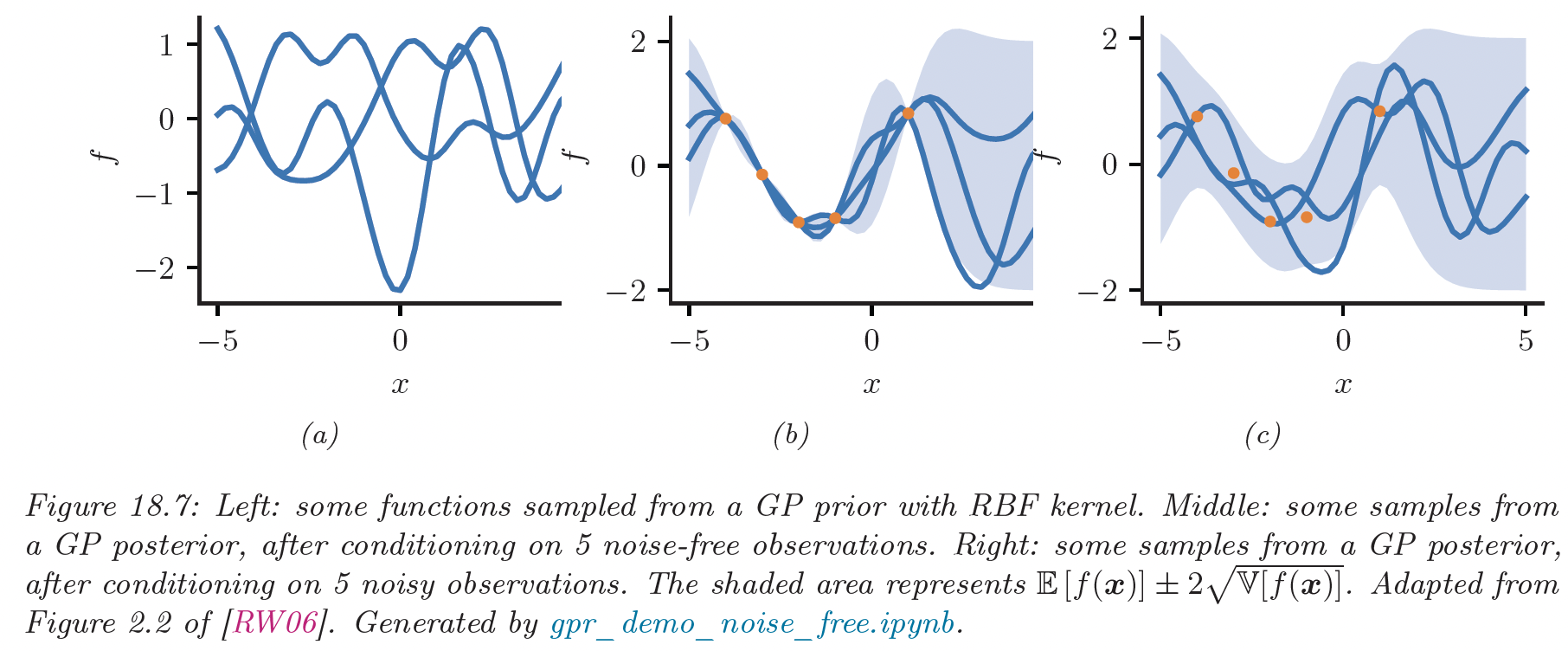
Example Posteriors (ProbML Book 2 Section 18.3.2)

Reproducing Kernel Hilbert Spaces (RKHS)

See ProbML Book 2 Section 18.3.7 for more details
Since we are working with function spaces, and there is an implicit inner product \(\phi(x)\) associated with the kernel \(\mathcal{K}(x,x')\)
We can construct a Hilbert Space using those inner products
- Denote the space \(\mathcal{H}_{\mathcal{K}}\) for kernel \(\mathcal{K}\)
- All inner product spaces induce a norm, so we can write \(||f||_{\mathcal{H}_{\mathcal{K}}}\)

ERM in a Function Space

ERM in a function space with LLS and a norm \(||f||\)

\[ \min_{f \in \mathcal{F}} \left\{\sum_{n=1}^N (y_n - f(x_n))^2 + \frac{\lambda}{2}||f||^2\right\} \]

If we use the RKHS function space associated with our kernel, we have the kernel ridge regression

\[ \min_{f \in \mathcal{H}_{\mathcal{K}}} \left\{\sum_{n=1}^N(y_n - f(x_n))^2 + \frac{\lambda}{2}||f||^2_{\mathcal{H}_{\mathcal{K}}}\right\} \]

Representer Theorem

See ProbML Book 2 Section 18.3.7.3 for more details
The representer theorem says that a solution to ERM in a function space

\[ f^* = \operatorname{argmin}_{f \in \mathcal{H}_{\mathcal{K}}} \left\{\sum_{n=1}^N\ell(f, x_n, y_n) + \frac{\lambda}{2}||f||^2_{\mathcal{H}_{\mathcal{K}}}\right\} \]
- Has a solution, for some coefficients \(\alpha_n\) a function of the data
\[ f^*(x) = \sum_{n=1}^N \alpha_n \mathcal{K}(x, x_n) \]
- See ProbML Book 2 for solutions for kernel ridge regression

Fitting GPs

Kernels themselves typically have parameters which must be fit/learned/etc. from the data
- e.g. the \(\ell\) bandwidth in the Gaussian kernel
This is typically done with maximum marginal likelihood or MAP
See ProbML Book 2 Section 18.3.5 and 18.6 for more details
Crucially, we can “learn the kernel” to mix representation learning with kernel methods/GPs

Manually Fitting a GP

Assume \(m(x) = 0\) for simplicity
Remember \(K_{XX} \equiv [K_{ij}]_{i,j=1}^N\) and \(\mathbf{\alpha}\equiv [\alpha_i]_{i=1}^N\) then, \[ ||f^*||^2_{\mathcal{H}_{\mathcal{K}}} = f^*\cdot f^* = \mathbf{\alpha}^{\top} K_{XX} \mathbf{\alpha} \]
Substitute into the Representer Theorem gives concrete optimization problem \[ \begin{aligned} &\min_{f \in \mathcal{H}_{\mathcal{K}}} \left\{\sum_{n=1}^N\ell(f, x_n, y_n) + \frac{\lambda}{2}||f||^2_{\mathcal{H}_{\mathcal{K}}}\right\}\\ &\min_{\mathbf{\alpha}} \left\{\sum_{n=1}^N\ell\left(\sum_{i=1}^N \alpha_n \mathcal{K}(x_n, x_i), x_n, y_n\right) + \frac{\lambda}{2}\mathbf{\alpha}^{\top} K_{XX}\mathbf{\alpha}\right\} \end{aligned} \]

Mean Functions and Hyperparameters

Kernels often have hyperparameters \(\theta\) (e.g., bandwidth) and parametric \(m(x;\eta, \theta)\)
Let \(K_{XX}(\theta) \equiv [K(x_i, x_j;\theta)]_{i,j=1}^N, \mathbf{x} \equiv [x_n]_{n=1}^N, \mathbf{y} \equiv [y_n]_{n=1}^N,\) and \(\mathbf{m}(\eta;\theta)\equiv [m(x;\theta, \eta)]_{n=1}^N\)
Often loss is written in terms of residuals, \(\mathbf{r}(f, \mathbf{x}, \mathbf{y})\) where \(\sum_{n=1}^N \ell(f, x_n, y_n) = ||\mathbf{r}(f, \mathbf{x}, \mathbf{y})||_2^2\)
- Then we can usually write the optimization problem as \[ \begin{aligned} \min_{\mathbf{\alpha}, \eta} &\left\{ ||\mathbf{r}(K_{XX}(\theta)\cdot \mathbf{\alpha}+ \mathbf{m}(\eta, \theta);\theta, \eta)||_2^2 + \frac{\lambda}{2}\mathbf{\alpha}^{\top}\cdot K_{XX}(\theta)\cdot\mathbf{\alpha}\right\}\\ \end{aligned} \]
- Then an outer optimization process for \(\theta\)!

Ridgeless Kernel Solution

Recall the min-norm, ridgeless OLS: \[ \lim_{\lambda \to 0} \operatorname{argmin}_{\alpha} ||\alpha \cdot X - y||^2_2 + \lambda ||\alpha||^2_2 = \operatorname{argmin}_{\alpha} ||\alpha||_2^2 \text{ s t. } \alpha \cdot X = y \]
With interpolating problem (i.e., \(\mathbf{r}(\cdot) = 0\) possible) take \(\lambda \to 0\) in Representer

\[ \begin{aligned} \min_{\mathbf{\alpha}, \eta} &\left\{\mathbf{\alpha}^{\top}K_{XX}(\theta)\mathbf{\alpha}\right\}\\ \text{s.t. }\, & \mathbf{r}(K_{XX}(\theta)\cdot \mathbf{\alpha}+ \mathbf{m}(\eta, \theta);\theta, \eta) = 0 \end{aligned} \]
- i.e. the min-norm (according to \(||f||_{\mathcal{H}_{\mathcal{K}}}\)) interpolating solution
- Can stack inequalities, additional constraints etc.
- With linear (in \(\mathcal{H}_{\mathcal{K}}\)) residuals/constraints can use very fast LQ solvers
- More explicit and reliable than the inductive bias in neural networks

GPytorch

One can manually create kernels and run the optimizer, or use a package such as GPyTorch
See examples/gpytorch_regression.py

import math
import torch
import gpytorch
from gpytorch.kernels import ScaleKernel, RBFKernel, LinearKernel
from matplotlib import pyplot as plt

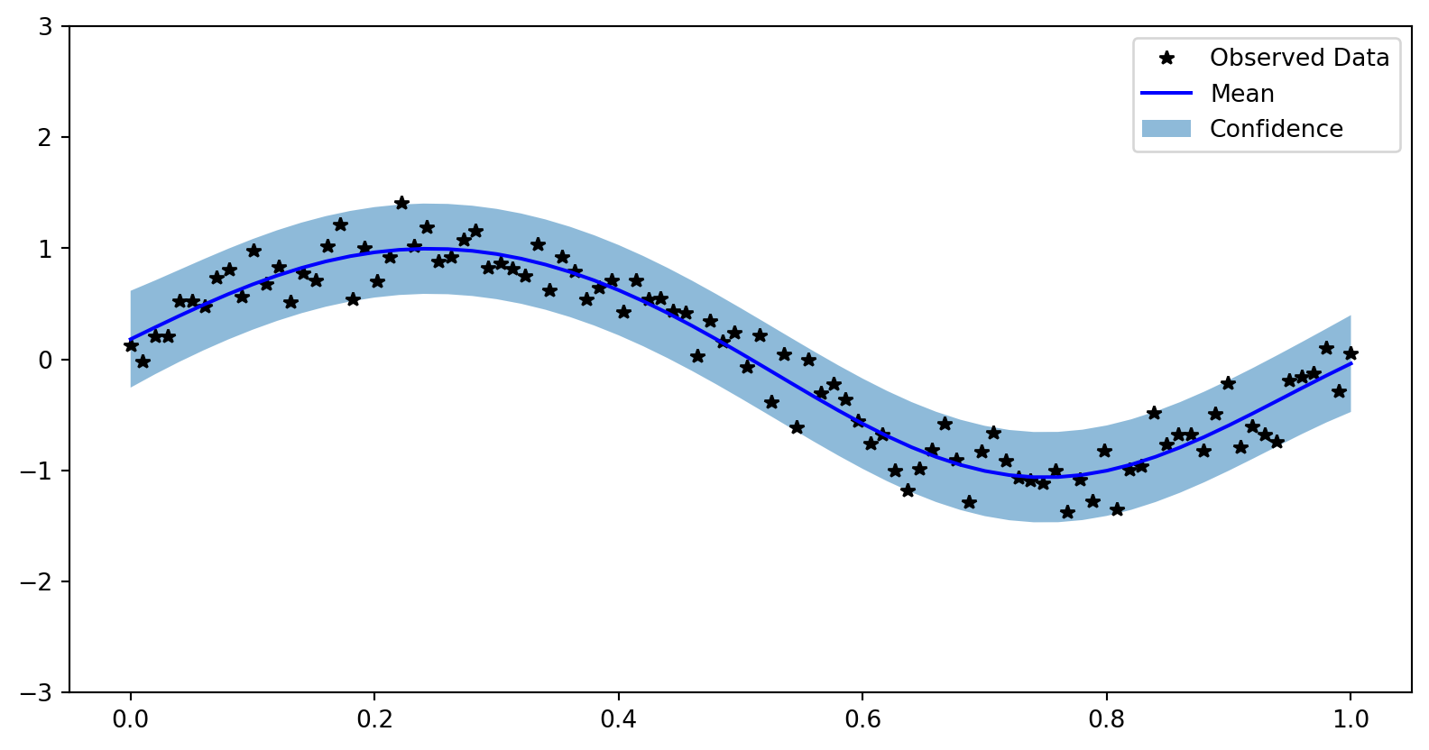
Example Training Data

# Training data is 100 points in [0,1] inclusive regularly spaced
train_x = torch.linspace(0, 1, 100)
# True function is sin(2*pi*x) with Gaussian noise
train_y = torch.sin(train_x * (2 * math.pi)) + torch.randn(train_x.size()) * math.sqrt(0.04)

Choosing Kernels

Kernels can be created from other kernels. e.g., given \(\mathcal{K}(x,x')\),
- \(\exp(\mathcal{K}(x,x'))\) is a valid kernel
- \(C \mathcal{K}(x,x')\) for a fixed scaling \(C > 0\)
- See the docs for more
Also, we can provide a “learnable” mean, \(m(x)\) for the process
- e.g. gpytorch.means.ConstantMean(), but could be function of \(x\)

Simple GP Model with exact inference

class ExactGPModel(gpytorch.models.ExactGP):
    def __init__(self, train_x, train_y, likelihood):
        super(ExactGPModel, self).__init__(train_x, train_y, likelihood)
        self.mean_module = gpytorch.means.ConstantMean()
        self.covar_module = gpytorch.kernels.ScaleKernel(gpytorch.kernels.RBFKernel())

    def forward(self, x):
        mean_x = self.mean_module(x)
        covar_x = self.covar_module(x)
        return gpytorch.distributions.MultivariateNormal(mean_x, covar_x)

Setup likelihood and Loss

likelihood = gpytorch.likelihoods.GaussianLikelihood()
model = ExactGPModel(train_x, train_y, likelihood)
model.train()
likelihood.train()
optimizer = torch.optim.Adam(model.parameters(), lr=0.1)  # Includes GaussianLikelihood parameters
# "Loss" for GPs - the marginal log likelihood
mll = gpytorch.mlls.ExactMarginalLogLikelihood(likelihood, model)
print(mll)

ExactMarginalLogLikelihood(
  (likelihood): GaussianLikelihood(
    (noise_covar): HomoskedasticNoise(
      (raw_noise_constraint): GreaterThan(1.000E-04)
    )
  )
  (model): ExactGPModel(
    (likelihood): GaussianLikelihood(
      (noise_covar): HomoskedasticNoise(
        (raw_noise_constraint): GreaterThan(1.000E-04)
      )
    )
    (mean_module): ConstantMean()
    (covar_module): ScaleKernel(
      (base_kernel): RBFKernel(
        (raw_lengthscale_constraint): Positive()
      )
      (raw_outputscale_constraint): Positive()
    )
  )
)

Run the Optimizer

for i in range(100):
    optimizer.zero_grad()
    # Output from model
    output = model(train_x)
    # Calc loss and backprop gradients
    loss = -mll(output, train_y)
    loss.backward()
    if i % 10 == 0:
      print(f"Iter={i}, Loss={loss.item()}")
    optimizer.step()
model.eval() # evaluation mode
likelihood.eval()

Iter=0, Loss=0.950839102268219
Iter=10, Loss=0.5059625506401062
Iter=20, Loss=0.16909293830394745
Iter=30, Loss=-0.05211631953716278
Iter=40, Loss=-0.04419197142124176
Iter=50, Loss=-0.05923301726579666
Iter=60, Loss=-0.06417526304721832
Iter=70, Loss=-0.06441757082939148
Iter=80, Loss=-0.06555411964654922
Iter=90, Loss=-0.06544952094554901

GaussianLikelihood(
  (noise_covar): HomoskedasticNoise(
    (raw_noise_constraint): GreaterThan(1.000E-04)
  )
)

Visualize Results

with torch.no_grad(), gpytorch.settings.fast_pred_var():
    test_x = torch.linspace(0, 1, 51)
    observed_pred = likelihood(model(test_x))

    fig, ax = plt.subplots()
    lower, upper = observed_pred.confidence_region()
    ax.plot(train_x.numpy(), train_y.numpy(), 'k*')
    ax.plot(test_x.numpy(), observed_pred.mean.numpy(), 'b')
    # Shade between the lower and upper confidence bounds
    ax.fill_between(test_x.numpy(), lower.numpy(), upper.numpy(), alpha=0.5)
    ax.set_ylim([-3, 3])
    ax.legend(['Observed Data', 'Mean', 'Confidence'])

Visualize Results