Introduction to Statistical Learning & Probabilistic Modeling
Machine Learning Fundamentals for Economists
Course Overview and Objectives
Course Overview
- First half of ECON 622: Computational Economics with Data Science Applications
- This section will cover a light version of important theory and methods from machine learning
- While we will cover applications, the emphasis will be on providing mathematical/statistical foundations to
- Understand these methods, and know their promises and limitations
- Adapt methods used in other disciplines to economic problems
- Want to understand deeply how these relate to classic methods like collocation
Textbooks
- All content in lecture notes, but some useful references from Kevin Murphy:
- See online PDFs and code at https://github.com/probml/pyprobml
- Also see Zhang et al. (2023)
- Provides more applied introduction with code examples in Python
Key Concepts and Topics
- Statistical Learning
- Supervised, unsupervised, self-supervised, generative
- Regularization and inductive bias
- Representation Learning (and Deep Learning)
- Feature learning vs. hand-crafted features
- Embeddings, geometry, and dimensionality reduction
- Transfer learning and reuse of representations
- High-Dimensional Optimization
- High-dimensional probability and concentration of measure
- Iterative and stochastic optimization methods
- Differentiation, forward- and reverse-mode autodiff
- Bayesian Methods and Uncertainty Quantification
Google AI Studio and Gemini API
- Sign up at aistudio.google.com
- There is a free tier with reasonable usage limits
- Later we will look at OpenAI and others
- Choose to “Get API key” in the sidebar (see here for details)
- Set
GEMINI_API_KEYas an environment variable
Python Packages
We will showcase a few examples using the Gemini API.
Calling an API
Generative AI uses algorithms to create new content, such as text, images, audio, and video, that resembles existing data but is not simply a copy of it.
Take 2: Context/Conditioning
Generative AI refers to algorithms and models that can create new, original content, such as text, images, audio, or code, based on the patterns and structures they learn from training data.
System Instructions (Persona)
In Gemini, “System Context” is a specific parameter in the configuration, ensuring the model adheres to the persona throughout the generation.
Generative artificial intelligence refers to a class of machine learning models capable of generating new, original content, such as text, images, audio, or other data, that resembles the data on which they were trained.
- For multi-step conversations, see Chat Example
Sampling Images
prompt = """
A comic-book stylized visualization
of mapping to an embedding manifold, showing data
points clustering in lower dimensions."""

response = client.models.generate_content(
    model="gemini-2.5-flash-image",
    contents=prompt,
    config=types.GenerateContentConfig(
        response_modalities=["IMAGE"]
    )
)
generated_img = response.parts[0].as_image()
display(IPImage(data=generated_img.image_bytes,
format='png'))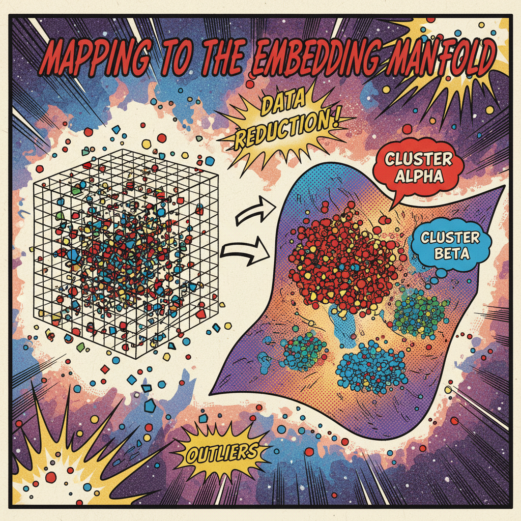
How is this Possible?
- The dimensionality of everything is enormous
- TOPIC Learn how to use these methods for traditional tasks
- e.g., classification and digitization as in Dell (2025)
- Is there any benefit for using related methods for solving more traditional economic problems?
- “Solving” functional equations with equilibrium conditions
- Estimating structural models
- Heterogeneous agent models
- causal inference (in second half of course)
- What is it actually doing, and how can we interpret it?
Statistical Learning and Functional Equations
Statistical Learning
Statistical learning studies how, given finite samples of random variables drawn from an underlying joint distribution, we can infer functions or probabilistic models that generalize beyond the observed sample
- Function (often used for prediction or decision): maps inputs/conditions to outputs.
- Examples: regression, classification, policy functions, surrogate mappings for PDE solution operators.
- Probabilistic model: represents uncertainty by modeling distributions.
- Examples: estimating conditional distributions; generative modeling; uncertainty quantification.
What is Prediction?
- “Predictive” does not mean “forecasting a time series,” and it does not imply a causal claim one way or another.
- It means the inferred object can be evaluated in some way on new, unseen realizations from the same (or a specified) population/joint distribution.
- For solving functional equations, it might mean that it has low residuals/errors on new states drawn from the same distribution as the training states.
Population Distribution
Observed “data” are realizations from an unknown population (data-generating) distribution
\[ (x, y) \sim \mu^* \]
- \(x \in {\mathcal{X}}\): inputs / features / covariates / states
- \(y \in {\mathcal{Y}}\): targets / labels / dependent variables
- As in ML and often in macro: abuse notation so \(x\) can be an RV or realization
- Typically \(\mu^*\) is unknown and only observed through samples
- For now, assume \(\mu^*\) is fixed (not innocuous, especially in econ applications)
In supervised learning, one object of interest is the conditional distribution \(y \mid x\)
- If solving a functional equation, \(y\) may be absent and we consider \(x \sim \mu^*\)
Risk Minimization
Many problems in ML, econometrics, and numerical analysis can be framed as finding a function \(f \in {\mathcal{F}}\) (e.g., a function, policy, or operator) such that \[ {f^*} = \arg\min_{f \in {\mathcal{F}}} \underbrace{\mathbb{E}_{(x,y)\sim \mu^*} \left[\ell(f, x, y)\right]}_{\equiv R(f, \mu^*)}. \]
One canonical example evaluates the squared error loss of “prediction” \[ {f^*} = \arg\min_{f \in {\mathcal{F}}} \mathbb{E}_{(x,y)\sim \mu^*} \left[\|y - f(x)\|_2^2\right]. \]
- This corresponds to modeling the conditional mean of \(y \mid x\)
Likelihoods and Population MLE
More generally, \(f\) may parameterize a full conditional distribution of \(y\) given \(x\) \[ {f^*} = \arg\min_{f \in {\mathcal{F}}} \mathbb{E}_{(x,y)\sim \mu^*} \left[-\log \mathbb{P}_f(y \mid x)\right]. \]
- This is population MLE for the conditional model \(\mathbb{P}_f(\cdot \mid x)\)
- Squared-error regression corresponds to a Gaussian likelihood with fixed variance
- Discrete-choice/classification corresponds to discrete conditional distributions
Equivalently, minimizes the expected KL divergence (see KL Divergence) \[ \mathbb{E}_{x\sim\mu^*} \mathrm{KL}\!\left(\mu^*(y\mid x)\,\|\,\mathbb{P}_f(y\mid x)\right), \]
Functional Equations
In many economic and numerical problems there is no target variable \(y\)
Instead, the goal is to find a function \(f \in {\mathcal{F}}\) satisfying conditions at each state \(x\) \[ {f^*} = \arg\min_{f \in {\mathcal{F}}} \mathbb{E}_{x\sim \mu^*} \left[\ell(f, x)\right]. \]
- The loss measures violations of a functional equation at state \(x\) (e.g., Euler errors)
If \(\ell({f^*}, x) = 0\) for all \(x \in {\mathcal{X}}\), then \({f^*}\) solves the functional equation pointwise
- We almost always assume such solutions exist.
- Risk minimization relaxes exact solution to an approximate solution in expectation, which is weaker.
Learning the \({f^*}\) or \(\mu^*(y \mid x)\)
- Outside of special cases, you cannot evaluate the objective directly.
- Several challenges:
- The population distribution \(\mu^*\) is unknown
- The function class \({\mathcal{F}}\) may be too rich to optimize over directly
- There may be (massive) multiplicity of functions which fulfill the objective
- In practice, we need to
- Use \({\mathcal{D}}\equiv \{((x_1, y_1), \ldots, (x_M, y_M))\}\subset {\mathcal{X}}\times {\mathcal{Y}}\)
- Restrict to a smaller “hypothesis class” \({\mathcal{H}}(\Theta) \subseteq {\mathcal{F}}\) with elements \(f_\theta\in {\mathcal{H}}(\Theta)\)
- Regularize directly or indirectly to choose among \(f_\theta\)
Empirical Risk Minimization (ERM)
Frequently, we will assume IID draws, \({\mathcal{D}}\overset{\mathrm{iid}}{\sim}\mu^*\), but this can be relaxed
The empirical counterpart to \(\arg\min_{f \in {\mathcal{F}}} \mathbb{E}_{(x,y)\sim \mu^*} \left[\ell(f, x, y)\right]\) is
\[ {\theta^*}\equiv \arg\min_{\theta \in \Theta}\underbrace{\frac{1}{|{\mathcal{D}}|}\sum_{(x,y) \in {\mathcal{D}}} \ell(f_{\theta}, x, y)}_{\equiv \hat{R}(\theta,{\mathcal{D}})} \]
- Variations: “regularization”, auxiliary objectives, constraints
- More advanced methods will also consider the sampling process for \({\mathcal{D}}\)
- TOPIC Especially challenging is when \(\mu^*(\cdot\,|\,{f^*})\), i.e., the distribution of future states in a macro model depends on the underlying policy
Example: Maximum Likelihood Estimation
The MLE case uses the negative log-likelihood loss \(\ell(f_\theta, x, y) = -\log \mathbb{P}_{\theta}(y \mid x)\)
The ERM objective becomes
\[ {\theta^*}= \arg\min_{\theta \in \Theta} \frac{1}{|{\mathcal{D}}|}\sum_{(x,y) \in {\mathcal{D}}} \left[-\log \mathbb{P}_{\theta}(y \mid x)\right] \]
- Common variations add regularization terms such as LASSO:
\[ {\theta^*}= \arg\min_{\theta \in \Theta} \frac{1}{|{\mathcal{D}}|}\sum_{(x,y) \in {\mathcal{D}}} \left[-\log \mathbb{P}_{\theta}(y \mid x)\right] + \lambda \|\theta\|_1 \]
- This may introduce bias since it no longer is the empirical version of the population MLE, but it may lead to better approximation on \({f^*}\) outside of \({\mathcal{D}}\).
Special Cases of MLE
- Regression: \(y \mid x \sim \mathcal{N}(f_\theta(x), \sigma^2) \Rightarrow\) least squares
- Classification: \(y \in \{1, \ldots, K\}\) with multinomial logit. See Zhang et al. (2023, sec. 4.1)
- “Softmax” in ML is just multinomial logit in econometrics
- Could be others (e.g., probit) but softmax is computationally convenient and has nie information theoretic properties
- Denote \(f_{\theta}(x)_k\) as the \(k\)-th element of the output vector then
Example: Functional Equations
Recall With \(x \in {\mathcal{X}}\), population risk minimization is \(\arg\min_{f \in {\mathcal{F}}}\mathbb{E}_{x\sim \mu^*} \left[\ell(f, x)\right]\)
Then the empirical problem is
\[ {\theta^*}= \arg\min_{\theta \in \Theta} \frac{1}{|{\mathcal{D}}|}\sum_{x \in {\mathcal{D}}} \ell(f_{\theta}, x) \]
- Typically there is interpolation and \(\ell(f_{{\theta^*}}, x) \approx 0\) for all \(x \in {\mathcal{D}}\)
- Nests collocation-style methods for solving functional equations
High-Dimensional Optimization
- TOPIC How can we optimize this in practice for
- high dimensional \({\mathcal{X}}\)
- large \(|{\mathcal{D}}|\)
- high-dimensional \(\theta\)
- complicated \(\ell(\cdot)\) and \(f_{\theta}\)
- e.g., stochastic optimization and iterative methods
- TOPIC How can we get gradients for optimization methods?
- e.g., \(\nabla_{\theta} \ell(f_{\theta}, x, y)\)
- Automatic differentiation (autodiff)
Clarity on our Goal
The optimization problem is a means-to-and-end:
- Want an \(f_{{\theta^*}}\) such that \(R(f_{{\theta^*}}, \mu^*)\) is as close to \(R({f^*}, \mu^*)\) as possible
- Solving ERM accurately is neither necessary nor sufficient for this purpose
TOPIC How well does a \(f_{{\theta^*}}\) approximate the population risk minimizer?
Crucially, this is not the same goal as minimizing the uniform error \[ \arg\min_{f \in {\mathcal{F}}} \max_{(x,y)\in {\mathcal{X}}\times{\mathcal{Y}}} \left[\ell(f, x, y)\right]. \]
- For low dimensional \((x,y)\) this may be possible, but…
Population vs. Empirical Risk
Population Risk
\[ {f^*}= \arg\min_{f \in {\mathcal{F}}} \underbrace{\mathbb{E}_{(x,y)\sim \mu^*} \left[\ell(f, x, y)\right]}_{\equiv R(f, \mu^*)} \]
Empirical Risk
\[ {\theta^*}= \arg\min_{\theta \in \Theta}\underbrace{\frac{1}{|{\mathcal{D}}|}\sum_{(x,y) \in {\mathcal{D}}} \ell(f_{\theta}, x, y)}_{\equiv \hat{R}(\theta,{\mathcal{D}})} \]
- Two separate sources of approximation error here (the bias-variance tradeoff):
- Approximation error \({\varepsilon_{\mathrm{app}}}\) (i.e. bias): \(f_{{\theta^*}} \in {\mathcal{H}}(\Theta)\) may not be able to represent \({f^*}\)
- Generalization error \({\varepsilon_{\mathrm{gen}}}\) (i.e. variance): Finite sample size of \({\mathcal{D}}\overset{\mathrm{iid}}{\sim}\mu^*\)
Error Decomposition
\[ \small \mathbb{E}_{{\mathcal{D}}\overset{\mathrm{iid}}{\sim}\mu^*}\left[\min_{\theta \in \Theta} \hat{R}(\theta, {\mathcal{D}}) - \min_{f \in \mathcal{F}} R(f, \mu^*)\right] = \underbrace{ R({f_{{\theta^*}}}, \mu^*) - R({f^*}, \mu^*)}_{\equiv {\varepsilon_{\mathrm{app}}}({f_{{\theta^*}}})} + \underbrace{\mathbb{E}_{{\mathcal{D}}\overset{\mathrm{iid}}{\sim}\mu^*}\left[\hat{R}(\theta^*, {\mathcal{D}}) - R({f_{{\theta^*}}}, \mu^*)\right]}_{\equiv {\varepsilon_{\mathrm{gen}}}({f_{{\theta^*}}})} \]
- TOPIC Modern ML shows we can often reduce both
- Will discuss the double-descent literature
- Punchline: simplicity leads to better generalization, but # parameters is poor heuristic for simplicity
- With a very flexible \({\mathcal{H}}(\Theta)\) such as neural networks often \({\varepsilon_{\mathrm{app}}}({f_{{\theta^*}}}) \approx 0\)
- Then error is \({\varepsilon_{\mathrm{gen}}}({f_{{\theta^*}}}) \approx \hat{R}(\theta^*, {\mathcal{D}}) - \hat{R}(\theta^*, {\mathcal{D}_{\mathrm{test}}})\) given new samples \({\mathcal{D}_{\mathrm{test}}}\overset{\mathrm{iid}}{\sim}\mu^*\)
Out-of-Sample vs. Out-of-Distribution
- Having a low \(\hat{R}({\theta^*}, {\mathcal{D}})\) is a means to an end, especially if \({\mathcal{D}}\) is measure zero in \({\mathcal{X}}\)
- Uniform errors (i.e., worst case \(x \in {\mathcal{X}}\)) are usually impossible with higher dimensions
- Out-of-Sample: consider \({\mathcal{D}_{\mathrm{test}}}\overset{\mathrm{iid}}{\sim}\mu^*\)
- Small \({\varepsilon_{\mathrm{gen}}}({f_{{\theta^*}}})\) means it generalizes well in-distribution
- Out-of-Distribution: consider \({\mathcal{D}}\sim \mu^*_1\) but \({\mathcal{D}_{\mathrm{test}}}\sim \mu^*_2\)
- If this generalizes well for reasonable \(\mu^*_2\) which are not too far from \(\mu^*_1\), we say it generalizes well out-of-distribution.
- TOPIC Robustness to distribution-shift is a major concern in practice
- e.g., if we solve a macro model with \({\mathcal{D}}\) generated from one discount factor, can we use the same samples to fit another?
Representations
Dimensionality with LLMs
- Consider the scale of generalization in modern deep learning
- Generative Pretrained Transformers (GPTs) approximate the conditional distribution of the next token
\[ \mathbb{P}\left[x_{T+1}\,|\,x_T, \ldots, x_1\right] \]
- Given a sequence \(x_1, \ldots, x_T\) of discrete random variables (tokens)
- Fit with variations on MLE over massive text corpora
LLM Scale
Frontier LLMs circa 2025: of \(K \approx 100{,}000\), context windows of \(T \approx 1{-}2\) million
GPT-4 class models: \(|\Theta| \approx 1{-}2\) trillion parameters approximating
\[ \mathbb{P} : \{1, \ldots, K\}^{T+1} \to [0,1], \quad K^{T+1} \approx (10^5)^{10^6} = 10^{5 \times 10^6} \]
- Trained on \(\approx 10{-}15\) trillion tokens of text data
- A tiny amount of data relative to the size of the function being approximated
Paraphrasing Belkin (2023): like reconstructing an entire library from a molecule of ink
They cannot possibly work on the entire space, or directly estimate \(\mathbb{P}\) as a table
Transformations of the Input
- Could approximate a function \(f(x)\) with a “shallow” approximation, e.g. polynomials of \(x\). Alternatively, nest functions \(h(\cdot)\) and \(\phi(\cdot)\) \[
f(x) \approx h(\phi(x))
\]
- First, the \(\phi(x)\) will transform the state into something more amenable for the downstream task (e.g. prediction, classification, etc.)
- Or, could include a fixed basis such as orthogonal polynomials
- Then the \(h(\cdot)\) maps that transformed state into the output.
- “Finding the State is an Art”
Some ML Terminology
- With \(h(\phi(x))\) they will often call these
- \(h(\cdot)\) the head or output layer
- \(\phi(\cdot)\) the feature map, encoder, or sometimes the backbone
- The representation \(\phi(x)\) is because it is often reused for multiple tasks
- Swap the “head” \(h(\cdot)\) but use the same \(\phi(x)\) - which is transferred
- Often \(\phi\) does not require re-estimated/learning and can be fixed
- Foundation models: a good \(\phi(\cdot)\) learned from a variety of different data sources that can be reused for many tasks
Latent State/Representation
- The \(\phi : {\mathcal{X}}\to {\mathcal{Z}}\) maps the original state \(x \in {\mathcal{X}}\) into a latent representation
- \({\mathcal{Z}}\) is often lower-dimensional than \({\mathcal{X}}\), but might be higher-dimensional
- If it has a interpretable norm, then often call it an embedding
- Then \(h : {\mathcal{Z}}\to {\mathcal{Y}}\) maps from the latent representation to the output
- Feature Engineering (i.e, “finding the state is an art”):
- Design \(\phi(\cdot)\) by hand (e.g., take means, logs, first-differences)
Notation for Parameters
- In many cases within ML there will be a collection of parameters for various parts of the functions
- We will denote the collection of all parameters as \(\theta \in \Theta\), where functions may only use a subset of those parameters
- e.g., \(\phi_{\theta}(x)\) and \(h_{\theta}(z)\) may use non-overlapping subsets of \(\theta\), or share them.
- This will become especially important when we consider gradients and optimization
- In some cases we may “freeze” the \(\theta_2\) in \(\theta \equiv \{\theta_1, \theta_2\}\) and only optimize over \(\theta_1\)
- In cases where a function does not have any parameters we might “learn” (i.e., optimize over) we will drop the subscript
Example: Polynomial Basis
Suppose \(x \in {\mathbb{R}}\) and we want to approximate \(f(x)\) with a polynomial of degree \(d\)
For some polynomial basis \(T_1(x), \ldots, T_d(x)\) (e.g., monomials, Chebyshev, Legendre, etc.) \[ \phi(x) = \begin{bmatrix}1 & T_1(x) & T_2(x) & \cdots & T_d(x)\end{bmatrix}^{\top} \]
- Note that there are no “learned” parameters!
Approximate \(f_{\theta}(x)\) with \(h_{\theta}(z) = W^{\top} z\), where \(W \in {\mathbb{R}}^{d+1}\) and \(W \in \theta\) \[ f_{\theta}(x) \equiv W^{\top} \phi(x) = \sum_{i=0}^d W_i T_i(x) \]
Example: Discrete-valued Probability Distributions
Recall cases of \(\mathbb{P}_{\theta}(y = k \mid x)\) for \(k \in \{1, \ldots, K\}\)
Stack the into a vector using \(\mathrm{softmax}: {\mathbb{R}}^K \to {\mathbb{R}}^K\) and pointwise \(\exp(\cdot)\)
\[ \mathrm{softmax}(z) \equiv \frac{\exp(z)}{\mathbf{1}^{\top}\exp(z)} \in {\mathbb{R}}^K, \quad \text{where } \mathbf{1}^{\top} \mathrm{softmax}(z) = 1 \]
Nesting the transformations with \(\phi_{\theta} : {\mathcal{X}}\to {\mathbb{R}}^L\) and head \(h_{\theta} : {\mathbb{R}}^L \to {\mathbb{R}}^K\)
\[ \mathbb{P}_{\theta}(y \mid x) = h_{\theta}(\phi_{\theta}(x)) \in {\mathbb{R}}^K \]
- \(\phi_{\theta} : {\mathcal{X}}\to {\mathbb{R}}^L\) is a nonlinear feature map to the latent space
- \(h_{\theta}(z) = \mathrm{softmax}(W z)\), where \(W \in {\mathbb{R}}^{K \times L}\) is part of \(\theta\)
Example: Functional Equations
- Recall ERM was \(\arg\min_{\theta \in \Theta} \frac{1}{|{\mathcal{D}}|}\sum_{x \in {\mathcal{D}}} \ell(f_{\theta}, x)\)
- Traditionally: use “shallow” approximation such as Chebyshev polynomials
- i.e., for \(f_{\theta}(x) = W^{\top} \phi(x)\) with \(\phi(x) \equiv \begin{bmatrix} 1 & T_0(x) & \cdots & T_d(x)\end{bmatrix}^{\top}\) on a grid \({\mathcal{D}}\subset {\mathcal{X}}\)
- Alternatively: change of variables to a better latent representation \[
f_{\theta}(x) = h_{\theta}(\phi_{\theta}(x))
\]
- With \(\phi_{\theta} : {\mathcal{X}}\to {\mathbb{R}}^L\) finding an efficient latent representation, and \(h_{\theta} : {\mathbb{R}}^L \to {\mathcal{Y}}\)
- These could be constructed (e.g., homotheticity) or “learned”
- Interpret \(\phi_{\theta}(\cdot)\) as an adaptive basis (see Wilson (2025))
Example: LLMs/Transformers
LLMs roughly build a latent representation \(\phi(\cdot)\) and \(h(\cdot)\)
\[ \mathbb{P}_{\theta}(y \mid x) = h_{\theta}(\phi_{\theta}(x)) \in {\mathbb{R}}^K \]
- \(\phi_{\theta}\) encodes the context \(\begin{bmatrix} x_1 & \ldots & x_T \end{bmatrix}\) into a latent vector \(z \in {\mathbb{R}}^L\)
- Design of \(\phi_{\theta}(\cdot)\) with LLMs uses the transformer architecture
- \(h_{\theta}(z) = \mathrm{softmax}(W z)\) with \(W \in {\mathbb{R}}^{K \times L}\)
- Output is the \(K\) simplex, \(\Delta_K \equiv \{p \in {\mathbb{R}}^{K}_+ : \sum_{k=1}^K p_k = 1\}\) (probability distributions over \(K\) values)
Once learned, \(\phi_{\theta}(\cdot)\) is useful for downstream tasks: embeddings, imputation, classification, etc.
Learning Representations
- Instead of hand-crafting \(\phi_{\theta}(\cdot)\), we can learn it from data
- TOPIC This process is called representation learning
- Good representations:
- Capture essential characteristics of the data
- Discard irrelevant information (compression/denoising)
- Orthogonalize sources of variation (disentanglement)
- Once learned, \(\phi_{\theta}(\cdot)\) is often reusable for multiple downstream tasks by fixing the \(\theta\)
Depth and Representation Learning
The mapping to outputs \(h(\cdot)\) is often “shallow” (e.g., linear or low-order polynomial)
In contrast, the transformation \(\phi(\cdot)\) into representation space is usually “deep”
\[ \phi \equiv \phi_L \circ \cdots \circ \phi_1 \]
As data becomes richer, unstructured, and higher-dimensional, transformations become harder to design manually
TOPIC Neural networks compose simple nonlinear functions to learn complicated transformations
- Depth leads to a combinatorial explosion in representational capacity
Representation Learning (Visual)
prompt = """
A stylized illustration of representation learning as a
smooth change of variables: a tangled, high-dimensional
data manifold being unfolded into a flat, low-dimensional
coordinate system. The left side shows intertwined curves
and knots; the right side shows clean, orthogonal axes
with separated clusters. Etching / wood-cut / scientific
engraving style, high contrast, minimal color palette."""
response = client.models.generate_content(
    model="gemini-2.5-flash-image",
    contents=prompt,
    config=types.GenerateContentConfig(
        response_modalities=["IMAGE"]
    )
)
generated_img = response.parts[0].as_image()
display(IPImage(data=generated_img.image_bytes,
format='png'))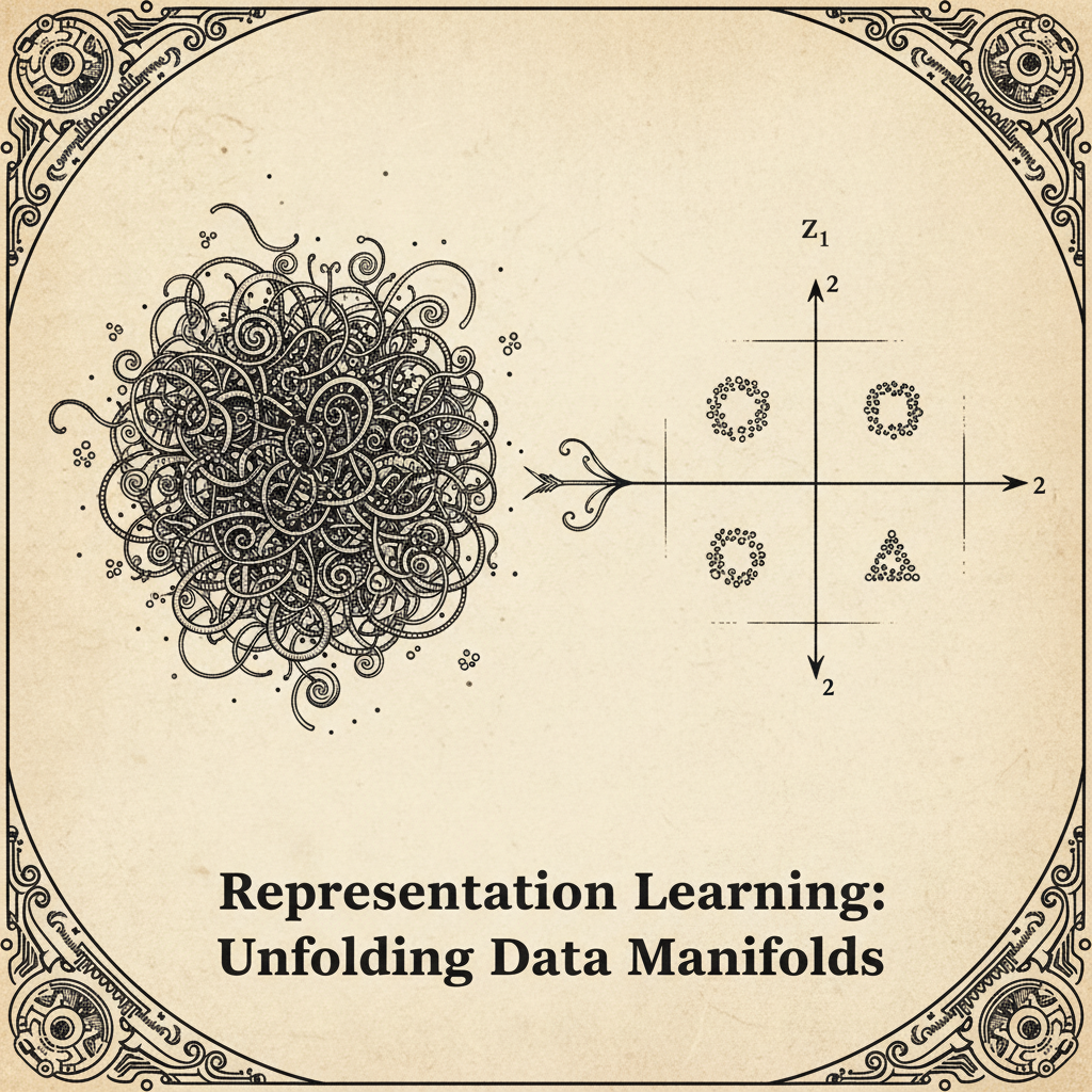
Representation Learning 2
prompt = """
An artistic visualization of representation learning
where entangled threads of data are transformed into
independent latent factors. On the left, a dense braid
of overlapping fibers; on the right, parallel strands
aligned along clear axes. Emphasize symmetry, order,
and factorization. Rendered in a vintage wood-engraving
or linocut style."""
response = client.models.generate_content(
    model="gemini-2.5-flash-image",
    contents=prompt,
    config=types.GenerateContentConfig(
        response_modalities=["IMAGE"]
    )
)
generated_img = response.parts[0].as_image()
display(IPImage(data=generated_img.image_bytes,
format='png'))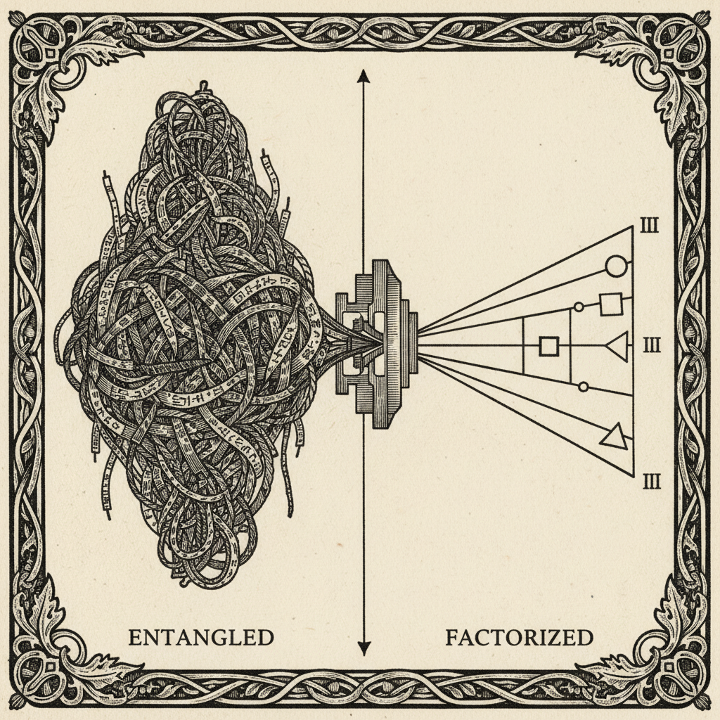
Representation Learning 3
prompt = """
A visual metaphor for representation learning as
 information compression: raw, noisy data clouds
 are compressed through a narrow bottleneck into
 a compact latent space that preserves structure.
 Before-and-after panels. Use engraved, chalkboard,
 or woodcut academic illustration style."""
response = client.models.generate_content(
    model="gemini-2.5-flash-image",
    contents=prompt,
    config=types.GenerateContentConfig(
        response_modalities=["IMAGE"]
    )
)
generated_img = response.parts[0].as_image()
display(IPImage(data=generated_img.image_bytes,
format='png'))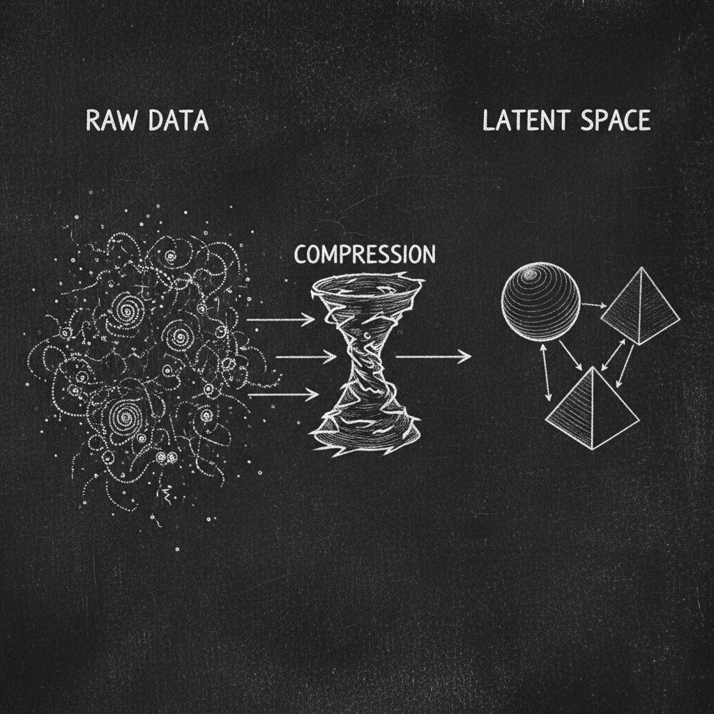
Representation Learning 4
prompt = """
A two-panel educational illustration explaining
representation learning. Left panel: high-dimensional,
entangled observations with overlapping features. Right
panel: low-dimensional latent representation with
disentangled, interpretable axes. Clean academic diagram
style with subtle wood-engraving texture."""
response = client.models.generate_content(
    model="gemini-2.5-flash-image",
    contents=prompt,
    config=types.GenerateContentConfig(
        response_modalities=["IMAGE"]
    )
)
generated_img = response.parts[0].as_image()
display(IPImage(data=generated_img.image_bytes,
format='png'))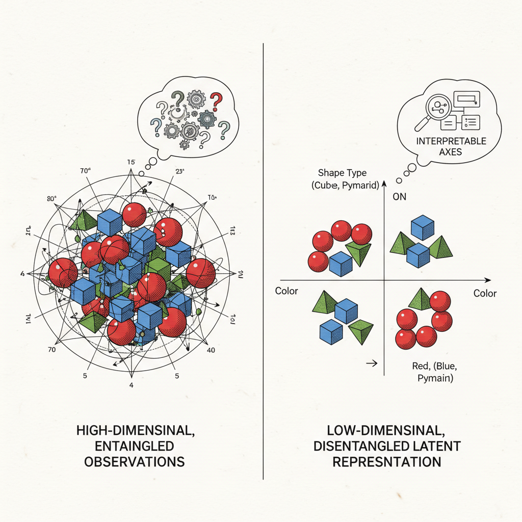
Computational Environment
Programming Languages
- Python
- “Raw” Numpy/skit-learn/etc.
- Torch, JAX, etc.
- Julia
- In this half we will focus on Python, but Julia has advantages in other areas.
Summary of Python Installation
See here for more details.
Clone Notebooks and Install Packages
- Open the command palette with
<Ctrl+Shift+P>or<Cmd+Shift+P>on mac and type> Git: Cloneand choosehttps://github.com/jlperla/grad_econ_ML_notebooks - In VS Code terminal in that repo,
uv sync - Then use VS Code to open any of the notebooks in that folder
Summary of Julia Installation
See here for more details.
- Install Git
- Install VS Code
- Install Julia following the Juliaup instructions
- Windows:
winget install julia -s msstorein a terminal - Linux/Mac:
curl -fsSL https://install.julialang.org | shin a terminal
- Windows:
- Install the VS Code Julia extension
Clone Notebooks and Install Packages
Open the command palette with
<Ctrl+Shift+P>or<Cmd+Shift+P>on mac and type> Git: Cloneand choosehttps://github.com/jlperla/grad_econ_ML_notebooksInstantiate packages by running VS Code terminal
] instantiate, where]enters package mode
Then use VS Code to open any of the notebooks in that folder
Note: the same clone’d repo can work for both Julia and Python
Appendices
Multi-step Conversations (Chat) Back
Use client.chats.create() to manage state. The chat object automatically tracks history so you don’t have to pass it back manually.
chat = client.chats.create(model=model, config=config)
res1 = chat.send_message("Describe the concept of generative AI in one sentence.")
print(f"Step 1: {res1.text}\n")

# Contextual follow-up
res2 = chat.send_message("Explain in one sentence how that relates to sampling from probability distributions.")
print(f"Step 2: {res2.text}")
Step 1: Generative artificial intelligence refers to a class of machine learning models that learn the underlying patterns and structure of input data and subsequently generate new data instances that plausibly could have been drawn from the same distribution.
Step 2: Generative AI models, after learning the probability distribution of the training data, effectively sample from that learned distribution to create new data points.
Population MLE and KL Divergence Back
Let \(\mu^*(y \mid x)\) denote the true conditional distribution, and \(\mathbb{P}_f(y \mid x)\) the model-implied conditional distribution
Take the the expected negative log-likelihood, condition on \(x\) and use the LIE \[ \begin{aligned} \mathbb{E}_{(x,y)\sim\mu^*} \left[-\log \mathbb{P}_f(y \mid x)\right] &= \mathbb{E}_{x\sim\mu^*} \left[ \mathbb{E}_{y\sim\mu^*(\cdot\mid x)} \left[-\log \mathbb{P}_f(y \mid x)\right] \right]. \end{aligned} \]
Add and subtract \(\log \mu^*(y \mid x)\) inside the inner expectation \[ \begin{aligned} &= \mathbb{E}_{x\sim\mu^*} \Big[ \underbrace{ \mathbb{E}_{y\sim\mu^*(\cdot\mid x)} \left[ \log \frac{\mu^*(y \mid x)}{\mathbb{P}_f(y \mid x)} \right] }_{\mathrm{KL}(\mu^*(y\mid x)\,\|\,\mathbb{P}_f(y\mid x))} & + \underbrace{ \mathbb{E}_{y\sim\mu^*(\cdot\mid x)} \left[-\log \mu^*(y \mid x)\right] }_{\text{does not depend on } f} \Big]. \end{aligned} \]
Therefore, minimizing expected log-loss is equivalent to minimizing KL \[ \mathbb{E}_{(x,y)\sim\mu^*} \left[-\log \mathbb{P}_f(y \mid x)\right] = \mathbb{E}_{x\sim\mu^*} \left[ \mathrm{KL}\!\left( \mu^*(y\mid x)\,\|\,\mathbb{P}_f(y\mid x) \right) \right] + \text{constant}. \]