High Dimensional Probability and Concentration of Measure

Machine Learning Fundamentals for Economists

Jesse Perla

jesse.perla@ubc.ca

University of British Columbia

Table of contents

• Overview
• High-Dimensional Geometry
• High Dimensional Probability
• When Concentration Fails
• Concentration is a Double-Edged Sword
• Random Algorithms in High Dimensions

Overview

Summary

• High-dimensional spaces exhibit counterintuitive geometric and probabilistic properties
• Key phenomena:
  • Curse of dimensionality: most volume is in corners, uniform sampling fails
  • Concentration of measure: functions of many variables are “essentially constant”
  • Johnson-Lindenstrauss: random projections preserve distances
  • Near-orthogonality: random vectors are almost perpendicular
  • Random algorithms: leverage concentration to provide probabilistic error guarantees
• These concepts are foundational for understanding why ML methods work
• Applications to solving structural economic models covered in subsequent lecture

References

• Primary reference: Vershynin (2018)
• Concentration inequalities: Boucheron, Lugosi, and Massart (2013)
• Classic reference: Ledoux (2001)

High-Dimensional Geometry

Hypercubes Are All Corners

• Counter-intuitive geometry: in high-dimensions, hypercubes are all corners
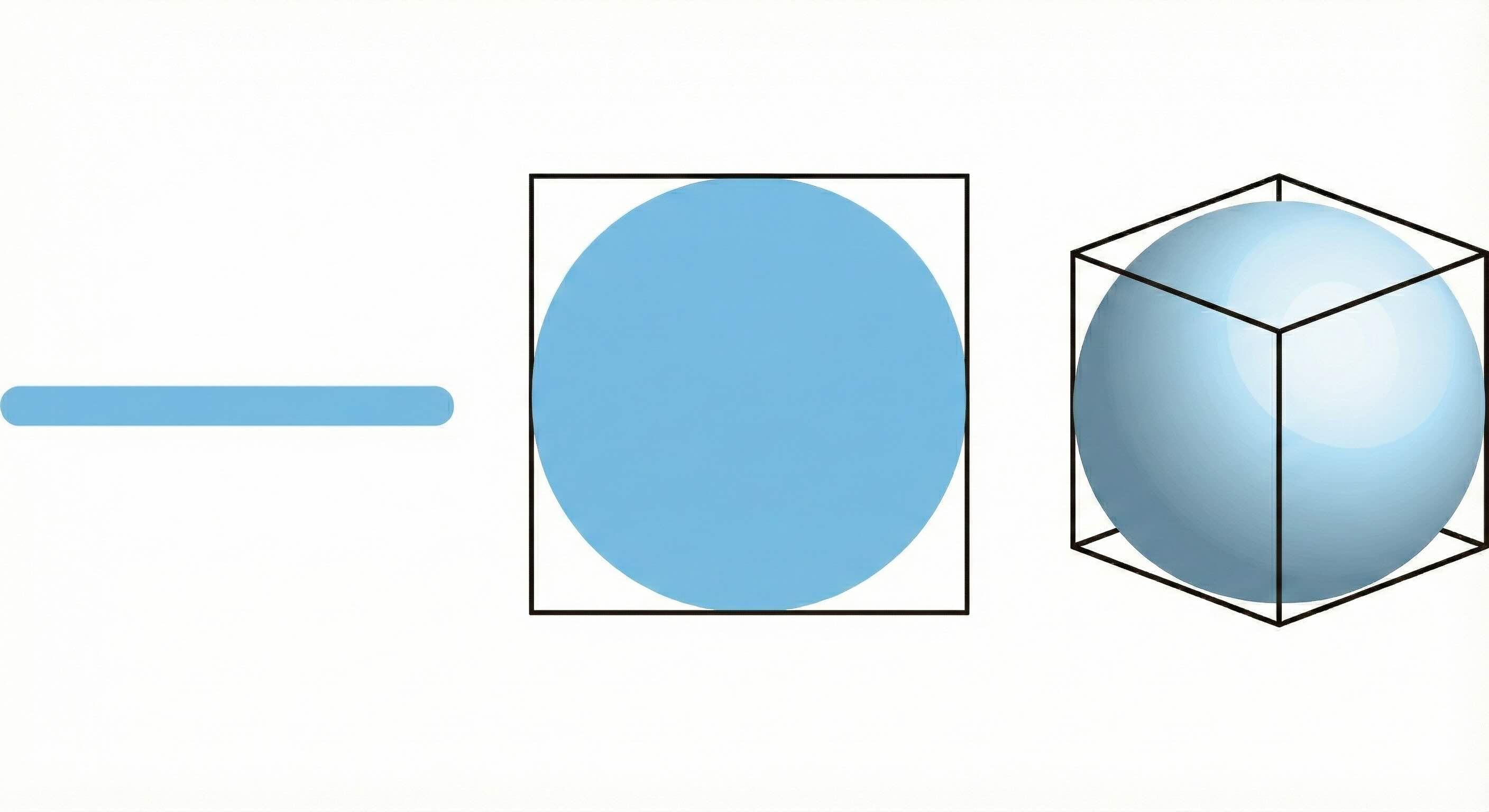
• Consider volume within a 1/2 radius of the origin in a hypercube \([-1/2,1/2]^N\)
  • Hypersphere inscribed in hypercube, touching all “faces” for all \(N\)
  • \(V(1) = 1\). The origin is close to every point on the line segment.
  • \(V(2) = \pi (1/2)^2, V(3) = \frac{4}{3} \pi (1/2)^3, V(10)\approx 0.002, V(50) = 1.536743\times 10^{-28}\)

• Largest possible sphere is vanishingly small!
• I think it touches \(N 2^{N-1}\) edges for \(N > 1\)

A High-Dimensional Space is a Lonely Place (Bernhard Schölkopf)

• Any \(X\) (e.g., steady-state) becomes increasingly distant from other regions of \({\mathcal{X}}\)
• Approximating functions with a grid or sampled on uniform \([X_{\min}, X_{\max}]^N\) distribution
  • Almost all of the volume in high-dimensional spaces is where you do not need it
  • i.e., not only does the num grid points, \(M\), need to increase exponentially with \(N\), but asymptotically almost every point is wasted for many applications
  • Calculating numerical expectations has similar issues (see Betancourt (2018))
• How could these possibly generalize from \({\mathcal{D}}\) to \({\mathcal{X}}\)? Is it really so hopeless?
  • ML and deep learning methods succeed in approximating functions on even richer spaces (e.g., images, videos, and NLP). Same with Bayesian methods like HMC.
  • Krusell-Smith approximations work very well in practice for many problems

• Similarly, how could you possibly calculate expectations? Most points in \(W_s\) would be in corners as well?
• Nearest neighbor becomes meaningless. The natural measure of distances is closer to a sliver in the right direction than to a ball.

High Dimensional Probability

Minimizing Uniform vs. Population Risk

• Uniform bounds on Errors: impossible in general without exponential cost in \(N\) \[ \min_{f\in {\mathcal{F}}}\sup_{(x,y) \in {\mathcal{X}}} \left[(f(x) - y)^2\right] \]

• Statistical learning: minimizes regions weighted by a distribution \(\mu^*\)

  \[ \min_{f \in {\mathcal{F}}} \mathbb{E}_{(x,y) \sim \mu^*}\left[(f(x) - y)^2\right] \]

  • Helps if probability distribution is “concentrated” in specific regions of \({\mathcal{X}}\)
  • Doesn’t help doesn’t if \(\mu^*\) is itself “all corners” (e.g., uniformly distributed)
  • Challenging if “worst case” matters (e.g., game with unconstrained best-responses)

Concentration of Measure Phenomenon

“A random variable that depends in a Lipschitz way on many independent variables (but not too much on any of them) is essentially constant.” (Ledoux (2001))

• i.e., functions of high-dimensional random variables have small variance if
  • The correlation between individual random variables are controlled
  • Lipshitz-like: If no single coordinate dominates, the function “averages out”
• Non-asymptotic bounds that improve with dimension (i.e., larger \(N\) is better, not worse)
• While geometry in \({\mathcal{X}}\) may be subject to a curse of dimensionality, functions of random variables on that space can become increasingly predictable

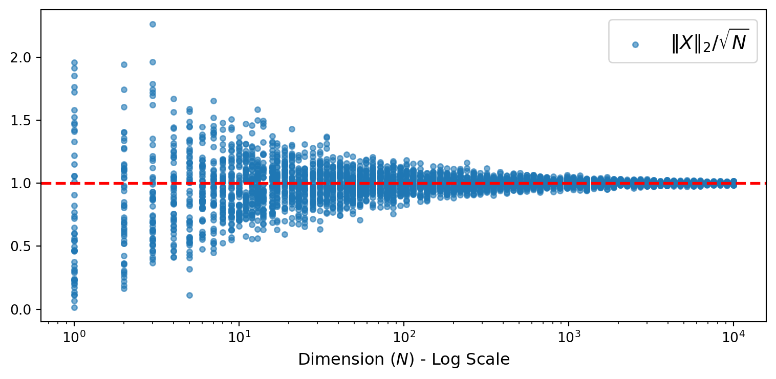
Example: Norm of Isotropic Gaussian

• Let \(X \sim \mathcal{N}(0_N, I_N)\) be an \(N\)-dimensional standard Gaussian
• Consider \(f(X) = \|X\|_2 / \sqrt{N}\)
• Can prove the concentration bound:

\[ {\mathbb{P}_{}\left( {|f(X) - 1| \geq \epsilon} \right)} \leq \exp(-c \epsilon^2 N) \]

for some constant \(c > 0\) independent of \(N\).

• The ratio \(\|X\|_2 / \sqrt{N}\) becomes increasingly predictable as \(N\) grows
• Convergence is exponentially fast in \(N\). Blessing, not curse, of dimensionality!

Visualization of Concentration of Norms

• 50 draws of \(X \sim \mathcal{N}(0_N, I_N)\) for each dimension \(N\)
• As \(N\) increases, all samples concentrate tightly around 1

The Soap Bubble Effect

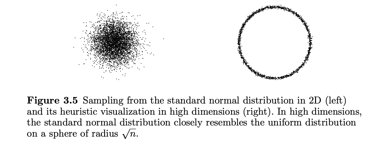
From Vershynin (2018): 2D Gaussian samples vs. random 2D projections of high-dimensional samples

• 2D Gaussians are distributed around the origin with an intuitive peak
• High-dim Gaussians are distributed roughly uniformly on a spherical shell of radius \(\sqrt{N}\)
• Points are nowhere near the mode/mean/median (i.e., \(X = 0_N\))

Lipschitz Concentration (Informal)

Definition: Lipschitz Function

A function \(f: {\mathbb{R}}^N \to {\mathbb{R}}\) is \(L\)-Lipschitz if for all \(x, y \in {\mathbb{R}}^N\):

\[ |f(x) - f(y)| \leq L \|x - y\|_2 \]

• Lipschitz functions cannot change too fast
• For \(f(x) = \|x\|_2\), we have \(L = 1\)
• Key insight: Lipschitz functions of Gaussians concentrate around their mean
• Can be extended to non-Lipschitz functions bounding expected gradients, etc.

Gaussian Concentration Inequality

Proposition: Concentration for Lipschitz Functions of Gaussians

Let \(X \sim \mathcal{N}(0_N, I_N)\) and let \(f: {\mathbb{R}}^N \to {\mathbb{R}}\) be \(L\)-Lipschitz. Then:

\[ {\mathbb{P}_{}\left( {|f(X) - \mathbb{E}[f(X)]| \geq t} \right)} \leq 2\exp\left(-\frac{t^2}{2L^2}\right) \]

• The bound is independent of dimension \(N\)!
• For normalized functions (gradient \(\mathrm{O}(1/\sqrt{N})\)), concentration improves with \(N\)
  • i.e., approximate average output of an industry vs. total output of an industry
• Many extensions: bounded differences, sub-Gaussian tails, etc. (Boucheron, Lugosi, and Massart (2013))

When Concentration Fails

Breaking Concentration: Three Mechanisms

The Gaussian concentration inequality requires:

1. Isotropic covariance: \(X \sim \mathcal{N}(0, I_N)\)
2. Lipschitz function: bounded gradient \(\|\nabla f\| \leq L\)
3. Distributed dependence: function doesn’t rely too heavily on any single coordinate

Violating (1) or (2) can break concentration, while violating (3) prevents improvement with dimension.

Operator Norm and Spectral Radius

Definition: Operator Norm and Spectral Radius

The operator norm (spectral norm) of \(A \in {\mathbb{R}}^{N \times N}\):

\[ {\left\| {A} \right\|_{\mathrm{op}}} = \sup_{x \neq 0} \frac{\|Ax\|_2}{\|x\|_2} \]

The spectral radius of \(A\):

\[ {\varrho\!\left( {A} \right)} = \max_i |\lambda_i(A)| \]

• In general: \({\varrho\!\left( {A} \right)} \leq {\left\| {A} \right\|_{\mathrm{op}}}\)
• For symmetric PSD matrices (e.g., covariance \(\Sigma\)): \({\left\| {\Sigma} \right\|_{\mathrm{op}}} = {\varrho\!\left( {\Sigma} \right)} = \lambda_{\max}(\Sigma)\)
• Concentration bounds depend on \({\varrho\!\left( {\Sigma} \right)}\): larger spectral radius → weaker concentration

Non-Isotropic Gaussians: The Setup

• Consider \(Z \sim \mathcal{N}(0, \Sigma)\) with general covariance \(\Sigma\)

• Write \(Z = \Sigma^{1/2} X\) where \(X \sim \mathcal{N}(0, I_N)\)

• For an \(L\)-Lipschitz function \(f\), define \(g(X) = f(\Sigma^{1/2} X)\)

  \[ |g(x) - g(y)| = |f(\Sigma^{1/2} x) - f(\Sigma^{1/2} y)| \leq L \|\Sigma^{1/2}(x-y)\|_2 \]

• Using operator norm: \(\|\Sigma^{1/2}(x-y)\|_2 \leq {\left\| {\Sigma^{1/2}} \right\|_{\mathrm{op}}} \|x-y\|_2 = \sqrt{{\varrho\!\left( {\Sigma} \right)}} \|x-y\|_2\)

Concentration with Non-Isotropic Gaussian

Proposition: Non-Isotropic Gaussian Concentration

For \(Z \sim \mathcal{N}(0, \Sigma)\) and \(f: {\mathbb{R}}^N \to {\mathbb{R}}\) that is \(L\)-Lipschitz:

\[ {\mathbb{P}_{}\left( {|f(Z) - \mathbb{E}[f(Z)]| \geq t} \right)} \leq 2\exp\left(-\frac{t^2}{2L^2 {\varrho\!\left( {\Sigma} \right)}}\right) \]

• The effective Lipschitz constant is \(L \sqrt{{\varrho\!\left( {\Sigma} \right)}}\)
• Concentration depends on the spectral radius of the covariance
• If \({\varrho\!\left( {\Sigma} \right)}\) grows with \(N\), concentration can degrade with dimension

Perfect Correlation Breaks Concentration

• Consider equicorrelation: \(\Sigma = \sigma^2\left((1-\rho)I_N + \rho \mathbf{1}_N \mathbf{1}_N^\top\right)\)
  • Diagonal: \(\Sigma_{ii} = \sigma^2\) (each variable has variance \(\sigma^2\))
  • Off-diagonal: \(\Sigma_{ij} = \sigma^2 \rho\) (correlation \(\rho\) between all pairs)
• Eigenvalues:
  • \(\sigma^2(1-\rho)\) with multiplicity \(N-1\)
  • \(\sigma^2(1 + (N-1)\rho)\) with multiplicity \(1\)
• As \(\rho \to 1\): \({\varrho\!\left( {\Sigma} \right)} \to \sigma^2 N\)

Perfect Correlation: The Bound Degrades

• With \({\varrho\!\left( {\Sigma} \right)} = \sigma^2 N\), the concentration bound becomes:

  \[ {\mathbb{P}_{}\left( {|f(Z) - \mathbb{E}[f(Z)]| \geq t} \right)} \leq 2\exp\left(-\frac{t^2}{2L^2 {\varrho\!\left( {\Sigma} \right)}}\right) = 2\exp\left(-\frac{t^2}{2L^2 \sigma^2 N}\right) \]

• Concentration gets worse with dimension!

• Intuition: With perfect correlation, all \(N\) variables move together

  • Effectively have only one degree of freedom, not \(N\)
  • No “averaging out” across independent sources of variation

• This is why independence (or weak dependence) is crucial for concentration

Functions of Single Coordinates

• Consider \(f(X) = X_1\) with \(X \sim \mathcal{N}(0, I_N)\)

• Gradient: \(\nabla f = (1, 0, \ldots, 0)^\top\), so \(L = 1\)

• Concentration bound:

  \[ {\mathbb{P}_{}\left( {|X_1| \geq t} \right)} \leq 2e^{-t^2/2} \]

• No improvement with dimension! The bound is the same for \(N = 10\) or \(N = 10{,}000\)

• \(X_1 \sim \mathcal{N}(0, 1)\) regardless of \(N\)—adding more coordinates doesn’t help

Contrast: Sample Mean Concentrates

• Compare with \(\bar{X} = \frac{1}{N}\sum_{i=1}^N X_i\)

• Gradient: \(\nabla \bar{X} = \frac{1}{N}(1, 1, \ldots, 1)^\top\)

• Lipschitz constant: \(L = \|\nabla \bar{X}\|_2 = \frac{1}{\sqrt{N}}\)

• Concentration bound:

  \[ {\mathbb{P}_{}\left( {|\bar{X}| \geq t} \right)} \leq 2\exp\left(-\frac{t^2 N}{2}\right) \]

• Improves with dimension! Exponentially tighter as \(N\) grows

• \(\bar{X} \sim \mathcal{N}(0, 1/N)\): variance shrinks as \(1/N\)

Key Insight: Coordinate Dependence

When Does Concentration Improve with \(N\)?

Concentration improves with dimension when no single coordinate dominates:

• \(\partial f / \partial X_i = \mathrm{O}(1/\sqrt{N})\) for all \(i\) → concentration improves
• \(\partial f / \partial X_1 = \mathrm{O}(1)\), others \(\approx 0\) → no improvement

• Intuition: The function must “average out” across many coordinates
• Functions that depend on all coordinates roughly equally benefit from high dimensions
• Functions concentrated on few coordinates behave like low-dimensional problems

Concentration is a Double-Edged Sword

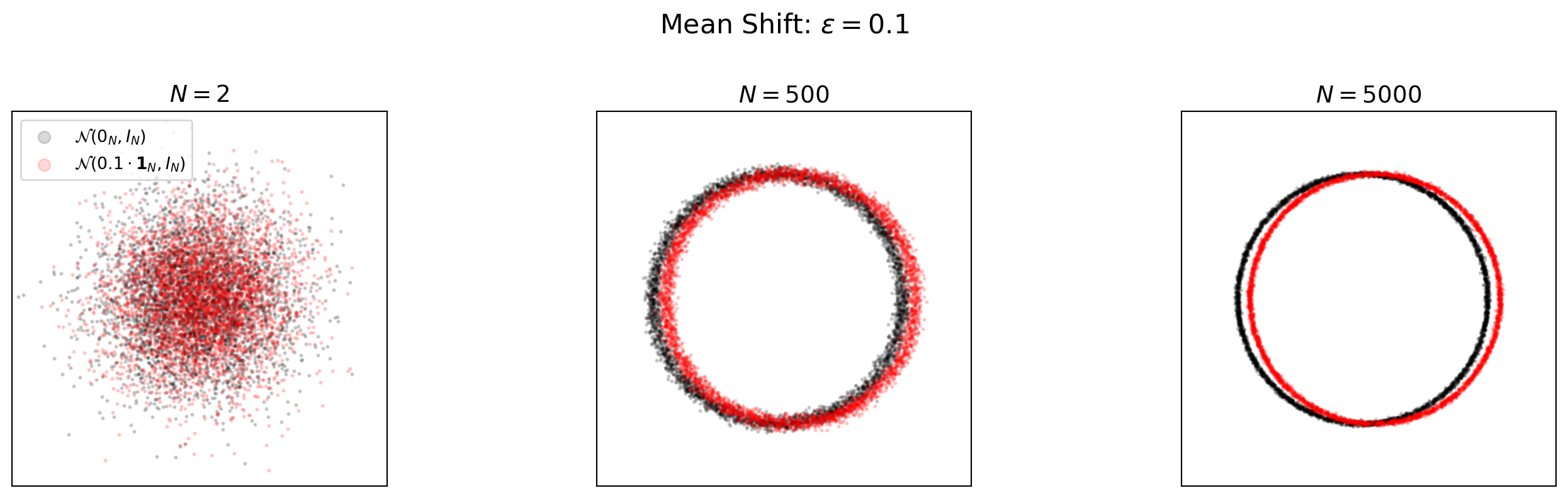
Shifted Mean: Increasing Separation

• Consider two distributions: \(\mathcal{N}(0_N, I_N)\) vs. \(\mathcal{N}(\epsilon \cdot \mathbf{1}_N, I_N)\)
• The Euclidean distance between means is \(\epsilon \sqrt{N}\)
• As \(N\) grows, distributions separate completely despite small per-coordinate shift
  • Showing random 2D projections from \(4000\) sampled points for visualization

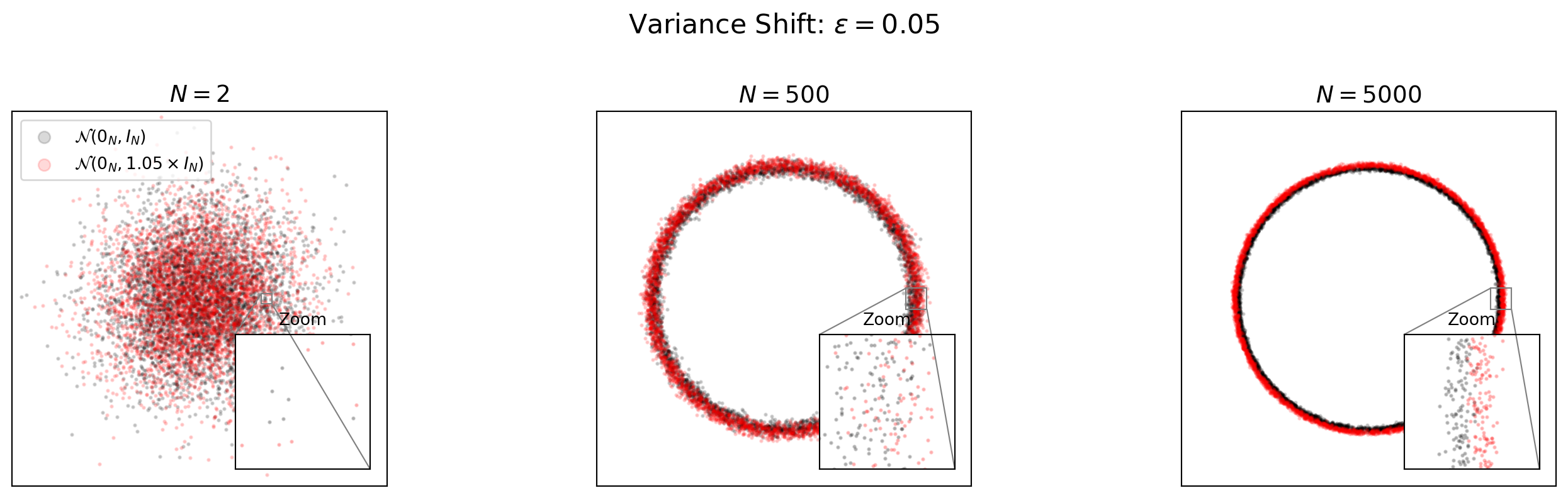
Variance Shift: Dangerous and Difficult to Detect

• Consider: \(\mathcal{N}(0_N, I_N)\) vs. \(\mathcal{N}(0_N, (1 + \epsilon) I_N)\)
• A 5% variance increase causes complete separation in high dimensions
  • Sampling more points from a slightly misspecified distribution may make statistical learning worse, not better.

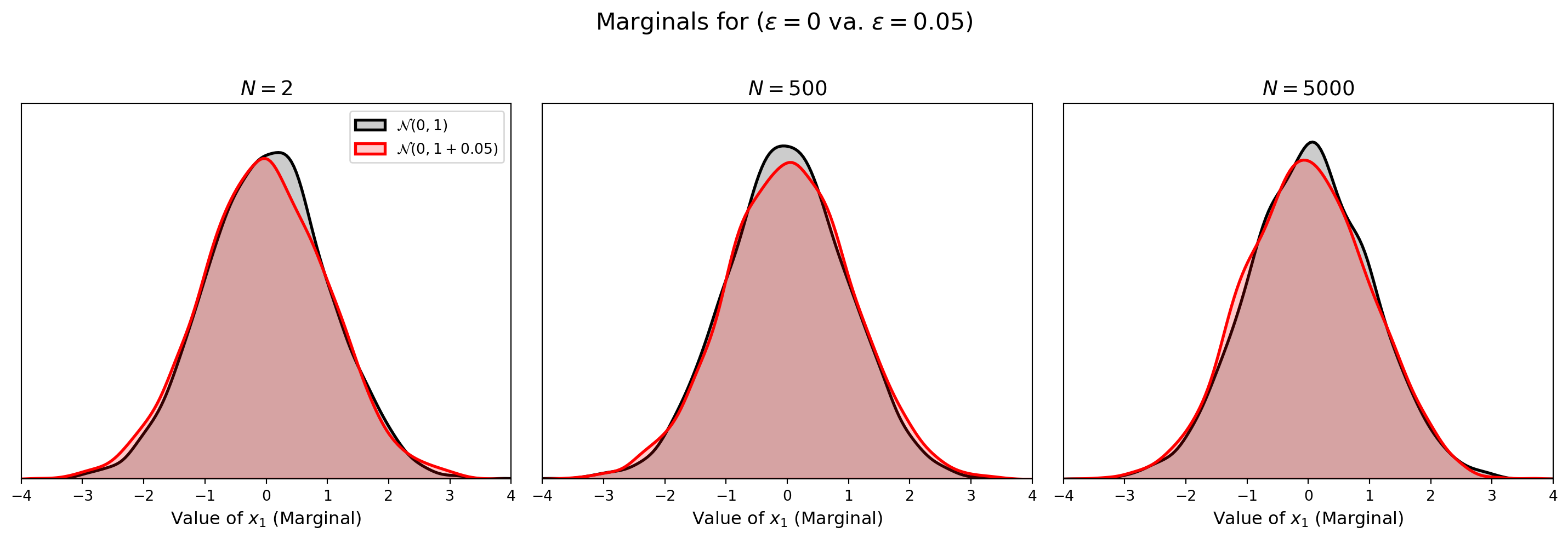
Marginals Are Deceptive

• With the shifted variance, the marginal distribution of any single coordinate is similar for both distributions
  • Showing the empirical 1D marginals of \(x_1\) from \(4000\) samples
• Recall that the joint distributions are completely separated in high dimensions

Key Insight: Double-Edged Sword

• Within a distribution: Concentration is helpful
  • Functions become predictable
  • Few samples may suffice for accurate estimation
• Across distributions: Concentration is dangerous
  • Small changes in distribution parameters cause complete separation
  • A model trained on one distribution may fail entirely on a slightly different one
• Implication for learning:
  • Must ensure training distribution \({\mathcal{D}}\sim \mu^*\) matches test distribution
  • “Out of distribution” generalization is fundamentally hard and requires changes to the training algorithm.
  • Representation learning becomes especially important. e.g., if functions were summarized well-approximated by mean and variance they could be learned and generalize well.

Random Algorithms in High Dimensions

Motivation

• High-dimensional economic models often involve objects that are:
  • Too large to store explicitly (e.g., large design or transition matrices)
  • Too costly to evaluate deterministically (e.g., integrals over \(\mathbb{R}^{100}\) or OLS with two-way fixed effects with millions of observations)
• Random algorithms use carefully designed randomness to:
  • Control approximation error probabilistically
  • Replace exponential complexity with polynomial or logarithmic complexity
• These are not heuristics—they satisfy non-asymptotic error bounds:
  • \(\mathbb{P}(|\text{Error}| > \epsilon) \le \delta\) where \(\delta\) includes functions of the number of samples, lipshitz constants, etc. Often decreasing, rather than increasing, in dimension \(N\)
  • Justified by concentration of measure

Johnson–Lindenstrauss as a Guiding Principle

Proposition: Johnson–Lindenstrauss (JL) Lemma

For any \(\epsilon \in (0,1)\), \(\delta \in (0,1)\), and points \(\{x_1,\dots,x_M\}\subset\mathbb{R}^N\), let \(R \in \mathbb{R}^{k \times N}\) be a random matrix (e.g., Gaussian or Rademacher entries) scaled by \(1/\sqrt{k}\). If

\[ k = \mathrm{O}\left(\epsilon^{-2} \log(M^2/\delta)\right), \]

then with probability at least \(1-\delta\), for all \(i,j\):

\[ (1-\epsilon)\|x_i-x_j\|_2^2 \;\le\; \|R x_i - R x_j\|_2^2 \;\le\; (1+\epsilon)\|x_i-x_j\|_2^2. \]

• Key insight: Randomness can preserve structure (i.e., geometry as captured by norms/similarity) uniformly over many objects
• JL provides a paradigm for probabilistic error control in random algorithms
• Other random algorithms share the same concentration foundation, but operate in different regimes of estimating functionals vs. preserving geometry

Why Does \(k\) Depend on \(M\), Not \(N\)?

• The projection dimension \(k\) depends on how many distances to preserve, not original dimension
• With 2 points: only 1 distance to preserve
  • Can project to \(k = \mathrm{O}(\epsilon^{-2})\) dimensions
  • A single projected distance concentrates around the true distance
• With \(M\) points: must preserve \(\binom{M}{2} = \mathrm{O}(M^2)\) distances simultaneously
  • Need \(k = \mathrm{O}(\epsilon^{-2} \log(M^2/\delta))\) for all to hold with failure probability at most \(\delta\)
  • The \(\log M\) factor comes from a union bound over all pairs

Why Random Projections Work: The Math

• Each individual distance concentrates:

  \[ {\mathbb{P}_{}\left( {\left|\|Rx\|_2^2 - \|x\|_2^2\right| > \epsilon \|x\|_2^2} \right)} \lesssim e^{-c \epsilon^2 k} \]

• Union bound over \(\mathrm{O}(M^2)\) pairs: multiply failure probability by \(M^2\)

• To keep total failure \(\leq \delta\): need \(e^{-c\epsilon^2 k} \cdot M^2 \leq \delta\)

• Solving: \(k \gtrsim \epsilon^{-2}(2\log M + \log(1/\delta)) = \epsilon^{-2} \log(M^2/\delta)\)

• Dimension \(N\) appears nowhere! Randomness “averages out” across all \(N\) coordinates

JL Preserves Fixed Sets, Not New Points

Important Limitation

JL preserves distances among a fixed set of points \(\{x_1, \ldots, x_M\}\).

It provides no guarantee for distances involving a new point \(x_{M+1}\).

• A new point would require either:
  • A fresh random projection, or
  • Adding it to the set and increasing \(k\) accordingly
• Implication: JL is ideal for static datasets, less so for streaming/online settings
• For adaptively chosen points, different techniques are needed (e.g., oblivious subspace embeddings)

A Taxonomy of Concentration-Based Random Algorithms

Algorithm type	What is preserved	Economic application
JL / Random Projections	Pairwise geometry / inner products	High-dimensional moment inequalities
Hutchinson Trace	Spectral trace / quadratic forms	Variance decomposition
Randomized SVD / Sketching	Low-rank structure	Factor models, macro-finance
Stochastic Trace Estimation	Operator traces	Continuous-time asset pricing

We now look at canonical economic applications.

Application: Kline, Saggio, and Sølvsten (2020)

• Goal: Decompose wage variance into worker and firm components
• Variance component: For coefficient vector \(\beta\), estimate \(\theta = \beta^{\top} A \beta\)
  • Matrix \(A\) selects which component (e.g., worker effects, firm effects, covariance)
• Key matrices:
  • Projection matrix: \(P = X(X^{\top}X)^{-1}X^{\top}\) (leverages \(P_{ii}\) for leave-out corrections)
  • Bias correction: \(B = (X^{\top}X)^{-1} A\) (combines design with component selector)
• Challenge: \(P\) and \(B\) are massive - cannot form explicitly

Kline, Saggio, and Sølvsten (2020): Why Traces?

• The naive plug-in \(\hat{\theta} = \hat{\beta}^{\top} A \hat{\beta}\) is biased:

\[ \mathbb{E}[\hat{\beta}^{\top} A \hat{\beta}] = \beta^{\top} A \beta + \sigma^2 \cdot \mathrm{Tr}(B) \]

• To debias: estimate \(\mathrm{Tr}(B)\) via Hutchinson’s trick with Rademacher vectors \(z_j \in \{\pm1\}^N\):

  \[ \mathrm{Tr}(B) = \mathbb{E}_{z}[z^\top B z] \approx \frac{1}{m}\sum_{j=1}^m z_j^\top (B z_j) \]

  • Only need one linear solve of \((X^{\top}X) (B z) = A z\) for \(B z\) per draw \(z\).
  • No explicit matrix required. Use preconditioned iterative solvers for high-dimensional design matrices (see iterative methods for more)

Application: Continuous-Time Asset Pricing and Stochastic Trace

• Consider a high-dimensional diffusion on state \(X_t \in \mathbb{R}^N\):

  \[ dX_t = \mu(X_t)\,dt + \sigma(X_t)\,dW_t, \quad X_t \in \mathbb{R}^N, \quad dW_t \in \mathbb{R}^K\quad \text{Brownian motion} \]

  • \(\mu : \mathbb{R}^N \to \mathbb{R}^N\) is the drift and \(\sigma : {\mathbb{R}}^N \to {\mathbb{R}}^{N \times K}\) is the volatility

• The infinitesimal generator, \(\mathcal{A}\), for this process is

  \[ \mathcal{A}f(X) = \mu(X)^\top \nabla f(X) + \frac{1}{2} {\mathrm{Tr}\left( {\sigma(X) \sigma(X)^\top\nabla^2 f(X)} \right)} \]

Hamilton-Jacobi-Bellman Equation (HJBE)

Simple HJBE for asset pricing,

\[ \rho V(X) = u(X) + \mathcal{A}V(X) = u(X) + \mu(X)^\top \nabla V(X) + \frac{1}{2} {\mathrm{Tr}\left( {\sigma(X) \sigma(X)^\top \nabla^2 V(X)} \right)}, \]

• Discount rate \(\rho > 0\)
• Utility function \(u : {\mathbb{R}}^N \to {\mathbb{R}}\)
• Subject to initial and boundary conditions/transversality

Random Algorithm for Diffusion Term

• Goal: Compute \({\mathrm{Tr}\left( {\sigma(X)\sigma(X)^{\top} \nabla^2 V(X)} \right)}\)

  • Direct computation is \(\mathrm{O}(N^2)\) - infeasible for large \(N\)
  • Use cyclic trace trick to get \({\mathrm{Tr}\left( {\sigma(X) \sigma(X)^\top \nabla^2 V(X)} \right)} = {\mathrm{Tr}\left( {\sigma(X)^\top \nabla^2 V(X) \, \sigma(X)} \right)}\)

• Hutchinson estimator: For \(z \sim \mathcal{N}(0, I_K)\), let \(w = \sigma(X) z \in \mathbb{R}^N\)

  \[ {\mathrm{Tr}\left( {\sigma(X)^\top \nabla^2 V(X) \, \sigma(X)} \right)} = \mathbb{E}_{w\sim \mathcal{N}(0, \sigma(X) \sigma(X)^\top)}[w^\top \nabla^2 V(X) \, w] \]

• Estimate with \(m\) samples (each with \(\mathrm{O}(N)\) cost): \[ {\mathrm{Tr}\left( {\sigma(X)^\top \nabla^2 V(X) \, \sigma(X)} \right)} \approx \frac{1}{m} \sum_{j=1}^m w_j \cdot \left(\nabla^2 V(X) \cdot w_j\right), \quad w_j \sim \mathcal{N}(0, \sigma(X) \sigma(X)^\top) \]

  • \(\nabla^2 V(X) \cdot w\) is a Hessian-Vector Product (hvp) - use AD such as JAX’s hvp

Application (IN PROGRESS): Chiong and Shum (2019)

• Goal: Estimate discrete-choice models with extremely high-dimensional regressors \(X^t \in \mathbb{R}^d\)

• Use random-projections to reduce dimension from \(d\) to \(k \ll d\)

• Estimation relies on cyclic monotonicity of choice probabilities

• Cyclic Monotonicity Inequalities: For any cycle \(t_1,\dots,t_L\):

  \[ \sum_{\ell=1}^L \big(X^{t_{\ell+1}}\beta - X^{t_\ell}\beta \big)^\top p^{t_\ell} \;\le\; 0. \]

  This yields a finite collection of inner-product inequalities in \(\beta\).

Random Projection in Chiong and Shum (2019)

Apply a random projection \(\widetilde X^t = R X^t\), with \(k \ll d\).

• The same estimator is run on projected data
• JL-type bounds ensure that the inner products defining the inequalities are preserved with high probability
• The feasibility region of the estimator is approximately unchanged

Note

Essence: One random projection must preserve many inequalities simultaneously — this is exactly the JL regime.

References

Betancourt, Michael. 2018. “Probabilistic Computation.” https://betanalpha.github.io/assets/case_studies/probabilistic_computation.html.

Boucheron, Stéphane, Gábor Lugosi, and Pascal Massart. 2013. Concentration Inequalities: A Nonasymptotic Theory of Independence. Oxford University Press.

Chiong, Khai Xiang, and Matthew Shum. 2019. “Random Projection Estimation of Discrete-Choice Models with Large Choice Sets.” Management Science 65 (1): 256–71. https://doi.org/10.1287/mnsc.2017.2928.

Kline, Patrick, Raffaele Saggio, and Mikkel Sølvsten. 2020. “Leave-Out Estimation of Variance Components.” Econometrica 88 (5): 1859–98. https://doi.org/10.3982/ECTA16410.

Ledoux, Michel. 2001. The Concentration of Measure Phenomenon. 89. American Mathematical Society.

Vershynin, Roman. 2018. High-Dimensional Probability: An Introduction with Applications in Data Science. Vol. 47. Cambridge university press.