ECON622: Problem Set 4

Authors

Affiliation

Jesse Perla, UBC

Jesse Perla

University of British Columbia

Packages

Add whatever packages you wish here

import numpy as np
import matplotlib.pyplot as plt
import scipy
import pandas as pd
import torch
import jax
import jax.numpy as jnp
from jax import grad, hessian
import torch.nn as nn
import torch.optim as optim
from jax import random
import optax
import jax_dataloader as jdl
from jax_dataloader.loaders import DataLoaderJAX
from flax import nnx
from openai import OpenAI
import wandb
import jsonargparse

Question 1: W&B Logging and CLI (JAX NNX)

For the linear regression examples with PyTorch we added in linear_regression_pytorch_logging.py logging and a CLI interface — which came for free with PyTorch Lightning.

In this question you will add in some of those features to the linear_regression_jax_nnx.py example.

Question 1.1: Add W&B Logging

Take the linear_regression_jax_nnx.py copied below for your convenience and:

1. Setup W&B properly
2. Add in logging of the train_loss at every step of the optimizer
3. Remove the other epoch printing, or try to log an epoch specific ||theta - theta_hat|| if you wish
4. Log the end ||theta - theta_hat|| at the end of the training

# MODIFY CODE HERE
import jax
import jax.numpy as jnp
from jax import random
import optax
import jax_dataloader as jdl
from jax_dataloader.loaders import DataLoaderJAX
from flax import nnx

N = 500  # samples
M = 2
sigma = 0.001
rngs = nnx.Rngs(42)
theta = random.normal(rngs(), (M,))
X = random.normal(rngs(), (N, M))
Y = X @ theta + sigma * random.normal(rngs(), (N,))  # Adding noise

def residual(model, x, y):
    y_hat = model(x)
    return (y_hat - y) ** 2

def residuals_loss(model, X, Y):
    return jnp.mean(
        jax.vmap(residual, in_axes=(None, 0, 0))(
            model, X, Y
        )
    )

model = nnx.Linear(M, 1, use_bias=False, rngs=rngs)

lr = 0.001
optimizer = nnx.Optimizer(
    model, optax.sgd(lr), wrt=nnx.Param
)

@nnx.jit
def train_step(model, optimizer, X, Y):
    def loss_fn(model):
        return residuals_loss(model, X, Y)
    loss, grads = nnx.value_and_grad(loss_fn)(model)
    optimizer.update(model, grads)
    return loss


num_epochs = 1000
batch_size = 512
dataset = jdl.ArrayDataset(X, Y)
train_loader = DataLoaderJAX(
    dataset, batch_size=batch_size, shuffle=True
)
for epoch in range(num_epochs):
    for X_batch, Y_batch in train_loader:
        loss = train_step(
            model, optimizer, X_batch, Y_batch
        )

    if epoch % 100 == 0:
        err = jnp.linalg.norm(
            theta - jnp.squeeze(model.kernel)
        )
        print(
            f"Epoch {epoch},"
            f"||theta - theta_hat|| = {err}"
        )

err = jnp.linalg.norm(
    theta - jnp.squeeze(model.kernel)
)
print(f"||theta - theta_hat|| = {err}")

import jax
import jax.numpy as jnp
from jax import random
import optax
import jax_dataloader as jdl
from jax_dataloader.loaders import DataLoaderJAX
from flax import nnx
import wandb

N = 500  # samples
M = 2
sigma = 0.001
rngs = nnx.Rngs(42)
theta = random.normal(rngs(), (M,))
X = random.normal(rngs(), (N, M))
Y = X @ theta + sigma * random.normal(rngs(), (N,))  # Adding noise

def residual(model, x, y):
    y_hat = model(x)
    return (y_hat - y) ** 2

def residuals_loss(model, X, Y):
    return jnp.mean(
        jax.vmap(
            residual, in_axes=(None, 0, 0)
        )(model, X, Y)
    )

model = nnx.Linear(
    M, 1, use_bias=False, rngs=rngs
)

lr = 0.001
optimizer = nnx.Optimizer(
    model, optax.sgd(lr), wrt=nnx.Param
)

@nnx.jit
def train_step(model, optimizer, X, Y):
    def loss_fn(model):
        return residuals_loss(model, X, Y)
    loss, grads = nnx.value_and_grad(loss_fn)(model)
    optimizer.update(model, grads)
    return loss

wandb.init(
    project="econ622_ps4", mode="offline"
)

num_epochs = 1000
batch_size = 512
dataset = jdl.ArrayDataset(X, Y)
train_loader = DataLoaderJAX(
    dataset, batch_size=batch_size, shuffle=True
)
for epoch in range(num_epochs):
    for X_batch, Y_batch in train_loader:
        loss = train_step(
            model, optimizer, X_batch, Y_batch
        )
        wandb.log({"train_loss": float(loss)})

theta_error = float(
    jnp.linalg.norm(
        theta - jnp.squeeze(model.kernel)
    )
)
wandb.log({"final_theta_error": theta_error})
print(f"||theta - theta_hat|| = {theta_error}")
wandb.finish()

Question 1.2: Add CLI Interface

Now, take the above code and copy it into a file named linear_regression_jax_cli.py.

We want to make it CLI ready:

• A package with many features, most of which you wouldn’t use directly, is jsonargparse. Besides the more advanced features like configuration files and the instantiation of classes/etc. as arguments, the main difference will be that it checks the types of arguments and converts them for you using python typehints.
• Alternatively, you can use the builtin Argparse or any other CLI framework

In that case, you can adapt the following code for your linear_regression_jax_cli.py:

import jsonargparse
def main_fn(lr: float = 0.001, N: int = 100):
    print(f"lr = {lr}, N = {N}")

if __name__ == "__main__":
     jsonargparse.CLI(main_fn)

Using your CLI

In either case, at that point you should be able to call this with python linear_regression_jax_cli.py and have it use all of the default values, python linear_regression_jax_cli.py --N=200 to change them, etc.

Either submit the file as part of the assignment or just paste the code into the notebook.

The key idea is to wrap the training code in a function with typed arguments, then use jsonargparse.CLI() to expose those arguments. See mlp_regression_jax_nnx_logging.py for a full working example.

# Save as linear_regression_jax_cli.py
import jax
import jax.numpy as jnp
from jax import random
import optax
import jax_dataloader as jdl
from jax_dataloader.loaders import DataLoaderJAX
from flax import nnx
import wandb
import jsonargparse

def fit_model(
    N: int = 500,
    M: int = 2,
    sigma: float = 0.001,
    lr: float = 0.001,
    num_epochs: int = 1000,
    batch_size: int = 512,
    seed: int = 42,
    wandb_mode: str = "offline",
):
    if wandb_mode != "disabled":
        wandb.init(project="econ622_ps4", mode=wandb_mode)

    rngs = nnx.Rngs(seed)
    theta = random.normal(rngs(), (M,))
    X = random.normal(rngs(), (N, M))
    Y = X @ theta + sigma * random.normal(rngs(), (N,))

    def residual(model, x, y):
        y_hat = model(x)
        return (y_hat - y) ** 2

    def residuals_loss(model, X, Y):
        return jnp.mean(
            jax.vmap(
                residual, in_axes=(None, 0, 0)
            )(model, X, Y)
        )

    model = nnx.Linear(
        M, 1, use_bias=False, rngs=rngs
    )
    optimizer = nnx.Optimizer(
        model, optax.sgd(lr), wrt=nnx.Param
    )

    @nnx.jit
    def train_step(model, optimizer, X, Y):
        def loss_fn(model):
            return residuals_loss(model, X, Y)
        loss, grads = nnx.value_and_grad(
            loss_fn
        )(model)
        optimizer.update(model, grads)
        return loss

    dataset = jdl.ArrayDataset(X, Y)
    train_loader = DataLoaderJAX(
        dataset,
        batch_size=batch_size,
        shuffle=True,
    )
    for epoch in range(num_epochs):
        for X_batch, Y_batch in train_loader:
            loss = train_step(
                model, optimizer,
                X_batch, Y_batch,
            )
            if wandb_mode != "disabled":
                wandb.log(
                    {"train_loss": float(loss)}
                )

    theta_error = float(
        jnp.linalg.norm(
            theta - jnp.squeeze(model.kernel)
        )
    )
    print(f"||theta - theta_hat|| = {theta_error}")
    if wandb_mode != "disabled":
        wandb.log({"final_theta_error": theta_error})
        wandb.finish()

if __name__ == "__main__":
    jsonargparse.CLI(fit_model)

Run with: python linear_regression_jax_cli.py --lr=0.01 --N=200 --wandb_mode=disabled

Question 1.3 (BONUS): W&B Sweep

Given the CLI you can now run a hyperparameter search. For this bonus problem, do a hyperparameter search over the --lr argument by following the W&B documentation.

To get you started, your sweep YAML might look something like this:

program: linear_regression_jax_cli.py
name: JAX Example
project: linear_regression_jax
description: JAX Sweep
method: random
parameters:
  lr:
    min: 0.0001
    max: 0.01

Here the method is changed from Bayes to random because otherwise we would need to provide a metric to optimize over. Feel free to adapt any of these settings.

If you successfully run a sweep then paste in your own YAML file here, and a screenshot of the W&B dashboard showing something about the sweep results.

Save the YAML above as sweep.yaml, then run:

# From the terminal:
# wandb sweep sweep.yaml
# wandb agent <sweep_id>

The sweep will launch multiple runs with different --lr values sampled from [0.0001, 0.01]. Check the W&B dashboard for parallel coordinates plots and run comparisons.

Question 2: PyTorch Neural Networks

In the repository you have code that does a linear regression with PyTorch: linear_regression_pytorch_sgd.py.

Question 2.1: Shallow MLP

Make a new file that does the same thing, but replace the nn.Linear(M, 1, bias=False) with code that gives a neural network with multiple layers. Maybe try:

M = 2 # loaded automatically in the code
num_width = 8  # You can hardcode or add to the template/yaml code
nn.Sequential(
    nn.Linear(M, num_width),
    nn.ReLU(),
    nn.Linear(num_width, 1, bias = False)
)

Sequential(
  (0): Linear(in_features=2, out_features=8, bias=True)
  (1): ReLU()
  (2): Linear(in_features=8, out_features=1, bias=False)
)

This is a network with one “hidden” layer. Try this for a very shallow network (e.g. num_width = 8) and see if it converges with Adam or SGD. It is OK if it does not! Don’t spend too much time with it.

import torch
import torch.nn as nn
import torch.optim as optim
from torch.utils.data import DataLoader, TensorDataset
from tqdm import tqdm

torch.manual_seed(42)

N = 500
M = 2
sigma = 0.001
theta = torch.randn(M)
X = torch.randn(N, M)
Y = X @ theta + sigma * torch.randn(N)

dataset = TensorDataset(X, Y)
batch_size = 16
train_loader = DataLoader(
    dataset, batch_size=batch_size, shuffle=True
)

def residuals(model, X, Y):
    Y_hat = model(X).squeeze()
    return ((Y_hat - Y) ** 2).mean()

num_width = 8
model = nn.Sequential(
    nn.Linear(M, num_width),
    nn.ReLU(),
    nn.Linear(num_width, 1, bias=False)
)

lr = 0.001
num_epochs = 1000
optimizer = optim.Adam(model.parameters(), lr=lr)

for epoch in tqdm(range(num_epochs), desc="Epochs"):
    for X_batch, Y_batch in train_loader:
        optimizer.zero_grad()
        loss = residuals(model, X_batch, Y_batch)
        loss.backward()
        optimizer.step()

print(f"Final loss: {residuals(model, X, Y).item():.6f}")

Epochs:   0%|          | 0/1000 [00:00<?, ?it/s]Epochs:   1%|          | 6/1000 [00:00<00:18, 52.83it/s]Epochs:   1%|          | 12/1000 [00:00<00:18, 54.51it/s]Epochs:   2%|▏         | 18/1000 [00:00<00:17, 55.13it/s]Epochs:   2%|▏         | 24/1000 [00:00<00:17, 55.51it/s]Epochs:   3%|▎         | 30/1000 [00:00<00:17, 55.70it/s]Epochs:   4%|▎         | 36/1000 [00:00<00:17, 55.94it/s]Epochs:   4%|▍         | 42/1000 [00:00<00:17, 56.03it/s]Epochs:   5%|▍         | 48/1000 [00:00<00:16, 56.07it/s]Epochs:   5%|▌         | 54/1000 [00:00<00:16, 56.10it/s]Epochs:   6%|▌         | 60/1000 [00:01<00:16, 56.09it/s]Epochs:   7%|▋         | 66/1000 [00:01<00:16, 56.16it/s]Epochs:   7%|▋         | 72/1000 [00:01<00:16, 56.11it/s]Epochs:   8%|▊         | 78/1000 [00:01<00:16, 56.14it/s]Epochs:   8%|▊         | 84/1000 [00:01<00:16, 56.18it/s]Epochs:   9%|▉         | 90/1000 [00:01<00:16, 56.14it/s]Epochs:  10%|▉         | 96/1000 [00:01<00:16, 56.22it/s]Epochs:  10%|█         | 102/1000 [00:01<00:15, 56.24it/s]Epochs:  11%|█         | 108/1000 [00:01<00:15, 56.31it/s]Epochs:  11%|█▏        | 114/1000 [00:02<00:15, 56.23it/s]Epochs:  12%|█▏        | 120/1000 [00:02<00:15, 55.51it/s]Epochs:  13%|█▎        | 126/1000 [00:02<00:15, 55.54it/s]Epochs:  13%|█▎        | 132/1000 [00:02<00:15, 55.69it/s]Epochs:  14%|█▍        | 138/1000 [00:02<00:15, 55.73it/s]Epochs:  14%|█▍        | 144/1000 [00:02<00:15, 55.71it/s]Epochs:  15%|█▌        | 150/1000 [00:02<00:15, 55.82it/s]Epochs:  16%|█▌        | 156/1000 [00:02<00:15, 55.85it/s]Epochs:  16%|█▌        | 162/1000 [00:02<00:14, 55.99it/s]Epochs:  17%|█▋        | 168/1000 [00:03<00:14, 56.08it/s]Epochs:  17%|█▋        | 174/1000 [00:03<00:14, 56.12it/s]Epochs:  18%|█▊        | 180/1000 [00:03<00:14, 56.17it/s]Epochs:  19%|█▊        | 186/1000 [00:03<00:14, 56.05it/s]Epochs:  19%|█▉        | 192/1000 [00:03<00:14, 56.01it/s]Epochs:  20%|█▉        | 198/1000 [00:03<00:14, 55.41it/s]Epochs:  20%|██        | 204/1000 [00:03<00:14, 55.60it/s]Epochs:  21%|██        | 210/1000 [00:03<00:14, 55.81it/s]Epochs:  22%|██▏       | 216/1000 [00:03<00:14, 55.85it/s]Epochs:  22%|██▏       | 222/1000 [00:03<00:13, 55.96it/s]Epochs:  23%|██▎       | 228/1000 [00:04<00:13, 55.89it/s]Epochs:  23%|██▎       | 234/1000 [00:04<00:13, 55.95it/s]Epochs:  24%|██▍       | 240/1000 [00:04<00:13, 55.87it/s]Epochs:  25%|██▍       | 246/1000 [00:04<00:13, 55.96it/s]Epochs:  25%|██▌       | 252/1000 [00:04<00:13, 55.97it/s]Epochs:  26%|██▌       | 258/1000 [00:04<00:13, 55.97it/s]Epochs:  26%|██▋       | 264/1000 [00:04<00:13, 55.97it/s]Epochs:  27%|██▋       | 270/1000 [00:04<00:13, 56.00it/s]Epochs:  28%|██▊       | 276/1000 [00:04<00:12, 56.05it/s]Epochs:  28%|██▊       | 282/1000 [00:05<00:12, 55.97it/s]Epochs:  29%|██▉       | 288/1000 [00:05<00:12, 56.04it/s]Epochs:  29%|██▉       | 294/1000 [00:05<00:12, 55.94it/s]Epochs:  30%|███       | 300/1000 [00:05<00:12, 56.00it/s]Epochs:  31%|███       | 306/1000 [00:05<00:12, 56.05it/s]Epochs:  31%|███       | 312/1000 [00:05<00:12, 56.05it/s]Epochs:  32%|███▏      | 318/1000 [00:05<00:12, 56.11it/s]Epochs:  32%|███▏      | 324/1000 [00:05<00:12, 56.06it/s]Epochs:  33%|███▎      | 330/1000 [00:05<00:11, 56.10it/s]Epochs:  34%|███▎      | 336/1000 [00:06<00:11, 56.05it/s]Epochs:  34%|███▍      | 342/1000 [00:06<00:11, 56.06it/s]Epochs:  35%|███▍      | 348/1000 [00:06<00:11, 56.11it/s]Epochs:  35%|███▌      | 354/1000 [00:06<00:11, 55.98it/s]Epochs:  36%|███▌      | 360/1000 [00:06<00:11, 55.98it/s]Epochs:  37%|███▋      | 366/1000 [00:06<00:11, 56.03it/s]Epochs:  37%|███▋      | 372/1000 [00:06<00:11, 56.06it/s]Epochs:  38%|███▊      | 378/1000 [00:06<00:11, 56.04it/s]Epochs:  38%|███▊      | 384/1000 [00:06<00:10, 56.12it/s]Epochs:  39%|███▉      | 390/1000 [00:06<00:10, 56.10it/s]Epochs:  40%|███▉      | 396/1000 [00:07<00:10, 56.01it/s]Epochs:  40%|████      | 402/1000 [00:07<00:10, 56.12it/s]Epochs:  41%|████      | 408/1000 [00:07<00:10, 55.94it/s]Epochs:  41%|████▏     | 414/1000 [00:07<00:10, 56.02it/s]Epochs:  42%|████▏     | 420/1000 [00:07<00:10, 56.05it/s]Epochs:  43%|████▎     | 426/1000 [00:07<00:10, 55.95it/s]Epochs:  43%|████▎     | 432/1000 [00:07<00:10, 56.01it/s]Epochs:  44%|████▍     | 438/1000 [00:07<00:10, 55.97it/s]Epochs:  44%|████▍     | 444/1000 [00:07<00:09, 56.04it/s]Epochs:  45%|████▌     | 450/1000 [00:08<00:09, 55.99it/s]Epochs:  46%|████▌     | 456/1000 [00:08<00:09, 56.03it/s]Epochs:  46%|████▌     | 462/1000 [00:08<00:09, 55.84it/s]Epochs:  47%|████▋     | 468/1000 [00:08<00:09, 55.98it/s]Epochs:  47%|████▋     | 474/1000 [00:08<00:09, 55.90it/s]Epochs:  48%|████▊     | 480/1000 [00:08<00:09, 55.98it/s]Epochs:  49%|████▊     | 486/1000 [00:08<00:09, 56.02it/s]Epochs:  49%|████▉     | 492/1000 [00:08<00:09, 56.03it/s]Epochs:  50%|████▉     | 498/1000 [00:08<00:08, 56.06it/s]Epochs:  50%|█████     | 504/1000 [00:09<00:08, 56.09it/s]Epochs:  51%|█████     | 510/1000 [00:09<00:08, 56.01it/s]Epochs:  52%|█████▏    | 516/1000 [00:09<00:08, 56.01it/s]Epochs:  52%|█████▏    | 522/1000 [00:09<00:08, 55.87it/s]Epochs:  53%|█████▎    | 528/1000 [00:09<00:08, 55.90it/s]Epochs:  53%|█████▎    | 534/1000 [00:09<00:08, 55.46it/s]Epochs:  54%|█████▍    | 540/1000 [00:09<00:08, 55.64it/s]Epochs:  55%|█████▍    | 546/1000 [00:09<00:08, 55.74it/s]Epochs:  55%|█████▌    | 552/1000 [00:09<00:08, 55.85it/s]Epochs:  56%|█████▌    | 558/1000 [00:09<00:07, 55.93it/s]Epochs:  56%|█████▋    | 564/1000 [00:10<00:07, 55.85it/s]Epochs:  57%|█████▋    | 570/1000 [00:10<00:07, 55.94it/s]Epochs:  58%|█████▊    | 576/1000 [00:10<00:07, 55.76it/s]Epochs:  58%|█████▊    | 582/1000 [00:10<00:07, 55.84it/s]Epochs:  59%|█████▉    | 588/1000 [00:10<00:07, 55.93it/s]Epochs:  59%|█████▉    | 594/1000 [00:10<00:07, 55.96it/s]Epochs:  60%|██████    | 600/1000 [00:10<00:07, 55.95it/s]Epochs:  61%|██████    | 606/1000 [00:10<00:07, 55.93it/s]Epochs:  61%|██████    | 612/1000 [00:10<00:06, 56.02it/s]Epochs:  62%|██████▏   | 618/1000 [00:11<00:06, 55.97it/s]Epochs:  62%|██████▏   | 624/1000 [00:11<00:06, 56.05it/s]Epochs:  63%|██████▎   | 630/1000 [00:11<00:06, 55.93it/s]Epochs:  64%|██████▎   | 636/1000 [00:11<00:06, 55.99it/s]Epochs:  64%|██████▍   | 642/1000 [00:11<00:06, 55.98it/s]Epochs:  65%|██████▍   | 648/1000 [00:11<00:06, 56.04it/s]Epochs:  65%|██████▌   | 654/1000 [00:11<00:06, 56.08it/s]Epochs:  66%|██████▌   | 660/1000 [00:11<00:06, 56.04it/s]Epochs:  67%|██████▋   | 666/1000 [00:11<00:05, 56.15it/s]Epochs:  67%|██████▋   | 672/1000 [00:12<00:05, 56.14it/s]Epochs:  68%|██████▊   | 678/1000 [00:12<00:05, 56.11it/s]Epochs:  68%|██████▊   | 684/1000 [00:12<00:05, 55.65it/s]Epochs:  69%|██████▉   | 690/1000 [00:12<00:05, 55.74it/s]Epochs:  70%|██████▉   | 696/1000 [00:12<00:05, 55.88it/s]Epochs:  70%|███████   | 702/1000 [00:12<00:05, 55.95it/s]Epochs:  71%|███████   | 708/1000 [00:12<00:05, 56.03it/s]Epochs:  71%|███████▏  | 714/1000 [00:12<00:05, 56.03it/s]Epochs:  72%|███████▏  | 720/1000 [00:12<00:04, 56.08it/s]Epochs:  73%|███████▎  | 726/1000 [00:12<00:04, 56.09it/s]Epochs:  73%|███████▎  | 732/1000 [00:13<00:04, 55.93it/s]Epochs:  74%|███████▍  | 738/1000 [00:13<00:04, 56.01it/s]Epochs:  74%|███████▍  | 744/1000 [00:13<00:04, 55.91it/s]Epochs:  75%|███████▌  | 750/1000 [00:13<00:04, 55.89it/s]Epochs:  76%|███████▌  | 756/1000 [00:13<00:04, 55.84it/s]Epochs:  76%|███████▌  | 762/1000 [00:13<00:04, 55.84it/s]Epochs:  77%|███████▋  | 768/1000 [00:13<00:04, 55.87it/s]Epochs:  77%|███████▋  | 774/1000 [00:13<00:04, 55.86it/s]Epochs:  78%|███████▊  | 780/1000 [00:13<00:03, 55.95it/s]Epochs:  79%|███████▊  | 786/1000 [00:14<00:03, 55.85it/s]Epochs:  79%|███████▉  | 792/1000 [00:14<00:03, 55.95it/s]Epochs:  80%|███████▉  | 798/1000 [00:14<00:03, 55.91it/s]Epochs:  80%|████████  | 804/1000 [00:14<00:03, 55.96it/s]Epochs:  81%|████████  | 810/1000 [00:14<00:03, 56.00it/s]Epochs:  82%|████████▏ | 816/1000 [00:14<00:03, 56.03it/s]Epochs:  82%|████████▏ | 822/1000 [00:14<00:03, 56.05it/s]Epochs:  83%|████████▎ | 828/1000 [00:14<00:03, 55.98it/s]Epochs:  83%|████████▎ | 834/1000 [00:14<00:02, 55.95it/s]Epochs:  84%|████████▍ | 840/1000 [00:15<00:02, 56.01it/s]Epochs:  85%|████████▍ | 846/1000 [00:15<00:02, 54.48it/s]Epochs:  85%|████████▌ | 852/1000 [00:15<00:02, 54.95it/s]Epochs:  86%|████████▌ | 858/1000 [00:15<00:02, 55.16it/s]Epochs:  86%|████████▋ | 864/1000 [00:15<00:02, 55.38it/s]Epochs:  87%|████████▋ | 870/1000 [00:15<00:02, 55.11it/s]Epochs:  88%|████████▊ | 876/1000 [00:15<00:02, 55.44it/s]Epochs:  88%|████████▊ | 882/1000 [00:15<00:02, 55.63it/s]Epochs:  89%|████████▉ | 888/1000 [00:15<00:02, 55.78it/s]Epochs:  89%|████████▉ | 894/1000 [00:15<00:01, 55.76it/s]Epochs:  90%|█████████ | 900/1000 [00:16<00:01, 55.78it/s]Epochs:  91%|█████████ | 906/1000 [00:16<00:01, 55.87it/s]Epochs:  91%|█████████ | 912/1000 [00:16<00:01, 55.75it/s]Epochs:  92%|█████████▏| 918/1000 [00:16<00:01, 55.72it/s]Epochs:  92%|█████████▏| 924/1000 [00:16<00:01, 55.76it/s]Epochs:  93%|█████████▎| 930/1000 [00:16<00:01, 55.93it/s]Epochs:  94%|█████████▎| 936/1000 [00:16<00:01, 56.01it/s]Epochs:  94%|█████████▍| 942/1000 [00:16<00:01, 56.04it/s]Epochs:  95%|█████████▍| 948/1000 [00:16<00:00, 56.06it/s]Epochs:  95%|█████████▌| 954/1000 [00:17<00:00, 55.85it/s]Epochs:  96%|█████████▌| 960/1000 [00:17<00:00, 55.61it/s]Epochs:  97%|█████████▋| 966/1000 [00:17<00:00, 55.40it/s]Epochs:  97%|█████████▋| 972/1000 [00:17<00:00, 55.59it/s]Epochs:  98%|█████████▊| 978/1000 [00:17<00:00, 55.69it/s]Epochs:  98%|█████████▊| 984/1000 [00:17<00:00, 55.70it/s]Epochs:  99%|█████████▉| 990/1000 [00:17<00:00, 55.74it/s]Epochs: 100%|█████████▉| 996/1000 [00:17<00:00, 51.11it/s]Epochs: 100%|██████████| 1000/1000 [00:17<00:00, 55.79it/s]

Final loss: 0.000001

Question 2.2: Deep MLP

Now replace this with a deeper and wider network by the same pattern. Maybe something like:

M = 2 # loaded automatically in the code
num_width = 256  # You can hardcode or add to the template/yaml code
nn.Sequential(
    nn.Linear(M, num_width),
    nn.ReLU(),
    nn.Linear(num_width, num_width),
    nn.ReLU(),
    nn.Linear(num_width, num_width),
    nn.ReLU(),
    nn.Linear(num_width, num_width),
    nn.ReLU(),
    nn.Linear(num_width, 1, bias = False)
)

Sequential(
  (0): Linear(in_features=2, out_features=256, bias=True)
  (1): ReLU()
  (2): Linear(in_features=256, out_features=256, bias=True)
  (3): ReLU()
  (4): Linear(in_features=256, out_features=256, bias=True)
  (5): ReLU()
  (6): Linear(in_features=256, out_features=256, bias=True)
  (7): ReLU()
  (8): Linear(in_features=256, out_features=1, bias=False)
)

Try to optimize this now and see if it fits well with this deeper network. If this is too slow, change the num_width or remove a layer to see if it helps.

torch.manual_seed(42)

N = 500
M = 2
sigma = 0.001
theta = torch.randn(M)
X = torch.randn(N, M)
Y = X @ theta + sigma * torch.randn(N)

dataset = TensorDataset(X, Y)
batch_size = 16
train_loader = DataLoader(
    dataset, batch_size=batch_size, shuffle=True
)

num_width = 256
model_deep = nn.Sequential(
    nn.Linear(M, num_width),
    nn.ReLU(),
    nn.Linear(num_width, num_width),
    nn.ReLU(),
    nn.Linear(num_width, num_width),
    nn.ReLU(),
    nn.Linear(num_width, num_width),
    nn.ReLU(),
    nn.Linear(num_width, 1, bias=False)
)

lr = 0.001
num_epochs = 1000
optimizer = optim.Adam(model_deep.parameters(), lr=lr)

for epoch in tqdm(range(num_epochs), desc="Epochs"):
    for X_batch, Y_batch in train_loader:
        optimizer.zero_grad()
        loss = residuals(model_deep, X_batch, Y_batch)
        loss.backward()
        optimizer.step()

print(f"Final loss: {residuals(model_deep, X, Y).item():.6f}")

Epochs:   0%|          | 0/1000 [00:00<?, ?it/s]Epochs:   0%|          | 2/1000 [00:00<01:10, 14.11it/s]Epochs:   0%|          | 4/1000 [00:00<01:03, 15.71it/s]Epochs:   1%|          | 6/1000 [00:00<01:00, 16.41it/s]Epochs:   1%|          | 8/1000 [00:00<00:58, 16.85it/s]Epochs:   1%|          | 10/1000 [00:00<00:58, 17.07it/s]Epochs:   1%|          | 12/1000 [00:00<00:57, 17.26it/s]Epochs:   1%|▏         | 14/1000 [00:00<00:56, 17.40it/s]Epochs:   2%|▏         | 16/1000 [00:00<00:56, 17.50it/s]Epochs:   2%|▏         | 18/1000 [00:01<00:55, 17.56it/s]Epochs:   2%|▏         | 20/1000 [00:01<00:55, 17.56it/s]Epochs:   2%|▏         | 22/1000 [00:01<00:55, 17.52it/s]Epochs:   2%|▏         | 24/1000 [00:01<00:55, 17.49it/s]Epochs:   3%|▎         | 26/1000 [00:01<00:55, 17.50it/s]Epochs:   3%|▎         | 28/1000 [00:01<00:55, 17.53it/s]Epochs:   3%|▎         | 30/1000 [00:01<00:55, 17.55it/s]Epochs:   3%|▎         | 32/1000 [00:01<00:55, 17.50it/s]Epochs:   3%|▎         | 34/1000 [00:01<00:55, 17.55it/s]Epochs:   4%|▎         | 36/1000 [00:02<00:55, 17.52it/s]Epochs:   4%|▍         | 38/1000 [00:02<00:54, 17.51it/s]Epochs:   4%|▍         | 40/1000 [00:02<00:54, 17.50it/s]Epochs:   4%|▍         | 42/1000 [00:02<00:54, 17.47it/s]Epochs:   4%|▍         | 44/1000 [00:02<00:54, 17.50it/s]Epochs:   5%|▍         | 46/1000 [00:02<00:54, 17.53it/s]Epochs:   5%|▍         | 48/1000 [00:02<00:54, 17.54it/s]Epochs:   5%|▌         | 50/1000 [00:02<00:54, 17.55it/s]Epochs:   5%|▌         | 52/1000 [00:02<00:54, 17.53it/s]Epochs:   5%|▌         | 54/1000 [00:03<00:54, 17.50it/s]Epochs:   6%|▌         | 56/1000 [00:03<00:53, 17.49it/s]Epochs:   6%|▌         | 58/1000 [00:03<00:54, 17.44it/s]Epochs:   6%|▌         | 60/1000 [00:03<00:53, 17.49it/s]Epochs:   6%|▌         | 62/1000 [00:03<00:53, 17.50it/s]Epochs:   6%|▋         | 64/1000 [00:03<00:53, 17.37it/s]Epochs:   7%|▋         | 66/1000 [00:03<00:53, 17.43it/s]Epochs:   7%|▋         | 68/1000 [00:03<00:53, 17.46it/s]Epochs:   7%|▋         | 70/1000 [00:04<00:53, 17.51it/s]Epochs:   7%|▋         | 72/1000 [00:04<00:52, 17.51it/s]Epochs:   7%|▋         | 74/1000 [00:04<00:53, 17.39it/s]Epochs:   8%|▊         | 76/1000 [00:04<00:53, 17.42it/s]Epochs:   8%|▊         | 78/1000 [00:04<00:52, 17.47it/s]Epochs:   8%|▊         | 80/1000 [00:04<00:52, 17.51it/s]Epochs:   8%|▊         | 82/1000 [00:04<00:52, 17.54it/s]Epochs:   8%|▊         | 84/1000 [00:04<00:52, 17.53it/s]Epochs:   9%|▊         | 86/1000 [00:04<00:52, 17.50it/s]Epochs:   9%|▉         | 88/1000 [00:05<00:52, 17.46it/s]Epochs:   9%|▉         | 90/1000 [00:05<00:52, 17.44it/s]Epochs:   9%|▉         | 92/1000 [00:05<00:51, 17.48it/s]Epochs:   9%|▉         | 94/1000 [00:05<00:51, 17.47it/s]Epochs:  10%|▉         | 96/1000 [00:05<00:51, 17.48it/s]Epochs:  10%|▉         | 98/1000 [00:05<00:51, 17.50it/s]Epochs:  10%|█         | 100/1000 [00:05<00:51, 17.53it/s]Epochs:  10%|█         | 102/1000 [00:05<00:51, 17.52it/s]Epochs:  10%|█         | 104/1000 [00:05<00:51, 17.50it/s]Epochs:  11%|█         | 106/1000 [00:06<00:51, 17.46it/s]Epochs:  11%|█         | 108/1000 [00:06<00:51, 17.46it/s]Epochs:  11%|█         | 110/1000 [00:06<00:50, 17.47it/s]Epochs:  11%|█         | 112/1000 [00:06<00:50, 17.47it/s]Epochs:  11%|█▏        | 114/1000 [00:06<00:50, 17.46it/s]Epochs:  12%|█▏        | 116/1000 [00:06<00:51, 17.32it/s]Epochs:  12%|█▏        | 118/1000 [00:06<00:50, 17.34it/s]Epochs:  12%|█▏        | 120/1000 [00:06<00:50, 17.41it/s]Epochs:  12%|█▏        | 122/1000 [00:07<00:50, 17.45it/s]Epochs:  12%|█▏        | 124/1000 [00:07<00:50, 17.45it/s]Epochs:  13%|█▎        | 126/1000 [00:07<00:49, 17.50it/s]Epochs:  13%|█▎        | 128/1000 [00:07<00:49, 17.49it/s]Epochs:  13%|█▎        | 130/1000 [00:07<00:49, 17.50it/s]Epochs:  13%|█▎        | 132/1000 [00:07<00:49, 17.51it/s]Epochs:  13%|█▎        | 134/1000 [00:07<00:49, 17.52it/s]Epochs:  14%|█▎        | 136/1000 [00:07<00:49, 17.55it/s]Epochs:  14%|█▍        | 138/1000 [00:07<00:49, 17.54it/s]Epochs:  14%|█▍        | 140/1000 [00:08<00:49, 17.52it/s]Epochs:  14%|█▍        | 142/1000 [00:08<00:49, 17.48it/s]Epochs:  14%|█▍        | 144/1000 [00:08<00:48, 17.52it/s]Epochs:  15%|█▍        | 146/1000 [00:08<00:48, 17.49it/s]Epochs:  15%|█▍        | 148/1000 [00:08<00:48, 17.53it/s]Epochs:  15%|█▌        | 150/1000 [00:08<00:48, 17.56it/s]Epochs:  15%|█▌        | 152/1000 [00:08<00:48, 17.56it/s]Epochs:  15%|█▌        | 154/1000 [00:08<00:48, 17.54it/s]Epochs:  16%|█▌        | 156/1000 [00:08<00:48, 17.55it/s]Epochs:  16%|█▌        | 158/1000 [00:09<00:47, 17.55it/s]Epochs:  16%|█▌        | 160/1000 [00:09<00:47, 17.53it/s]Epochs:  16%|█▌        | 162/1000 [00:09<00:47, 17.53it/s]Epochs:  16%|█▋        | 164/1000 [00:09<00:47, 17.53it/s]Epochs:  17%|█▋        | 166/1000 [00:09<00:47, 17.52it/s]Epochs:  17%|█▋        | 168/1000 [00:09<00:47, 17.39it/s]Epochs:  17%|█▋        | 170/1000 [00:09<00:47, 17.42it/s]Epochs:  17%|█▋        | 172/1000 [00:09<00:47, 17.46it/s]Epochs:  17%|█▋        | 174/1000 [00:09<00:47, 17.51it/s]Epochs:  18%|█▊        | 176/1000 [00:10<00:47, 17.48it/s]Epochs:  18%|█▊        | 178/1000 [00:10<00:46, 17.53it/s]Epochs:  18%|█▊        | 180/1000 [00:10<00:46, 17.53it/s]Epochs:  18%|█▊        | 182/1000 [00:10<00:46, 17.47it/s]Epochs:  18%|█▊        | 184/1000 [00:10<00:46, 17.49it/s]Epochs:  19%|█▊        | 186/1000 [00:10<00:46, 17.48it/s]Epochs:  19%|█▉        | 188/1000 [00:10<00:46, 17.50it/s]Epochs:  19%|█▉        | 190/1000 [00:10<00:46, 17.50it/s]Epochs:  19%|█▉        | 192/1000 [00:11<00:46, 17.45it/s]Epochs:  19%|█▉        | 194/1000 [00:11<00:46, 17.41it/s]Epochs:  20%|█▉        | 196/1000 [00:11<00:46, 17.47it/s]Epochs:  20%|█▉        | 198/1000 [00:11<00:45, 17.45it/s]Epochs:  20%|██        | 200/1000 [00:11<00:45, 17.50it/s]Epochs:  20%|██        | 202/1000 [00:11<00:45, 17.52it/s]Epochs:  20%|██        | 204/1000 [00:11<00:45, 17.54it/s]Epochs:  21%|██        | 206/1000 [00:11<00:45, 17.55it/s]Epochs:  21%|██        | 208/1000 [00:11<00:45, 17.56it/s]Epochs:  21%|██        | 210/1000 [00:12<00:44, 17.58it/s]Epochs:  21%|██        | 212/1000 [00:12<00:44, 17.56it/s]Epochs:  21%|██▏       | 214/1000 [00:12<00:44, 17.58it/s]Epochs:  22%|██▏       | 216/1000 [00:12<00:44, 17.54it/s]Epochs:  22%|██▏       | 218/1000 [00:12<00:44, 17.53it/s]Epochs:  22%|██▏       | 220/1000 [00:12<00:44, 17.50it/s]Epochs:  22%|██▏       | 222/1000 [00:12<00:44, 17.51it/s]Epochs:  22%|██▏       | 224/1000 [00:12<00:44, 17.38it/s]Epochs:  23%|██▎       | 226/1000 [00:12<00:44, 17.38it/s]Epochs:  23%|██▎       | 228/1000 [00:13<00:44, 17.46it/s]Epochs:  23%|██▎       | 230/1000 [00:13<00:44, 17.47it/s]Epochs:  23%|██▎       | 232/1000 [00:13<00:43, 17.49it/s]Epochs:  23%|██▎       | 234/1000 [00:13<00:43, 17.47it/s]Epochs:  24%|██▎       | 236/1000 [00:13<00:43, 17.47it/s]Epochs:  24%|██▍       | 238/1000 [00:13<00:43, 17.46it/s]Epochs:  24%|██▍       | 240/1000 [00:13<00:43, 17.50it/s]Epochs:  24%|██▍       | 242/1000 [00:13<00:43, 17.52it/s]Epochs:  24%|██▍       | 244/1000 [00:13<00:43, 17.56it/s]Epochs:  25%|██▍       | 246/1000 [00:14<00:43, 17.53it/s]Epochs:  25%|██▍       | 248/1000 [00:14<00:43, 17.44it/s]Epochs:  25%|██▌       | 250/1000 [00:14<00:42, 17.46it/s]Epochs:  25%|██▌       | 252/1000 [00:14<00:42, 17.47it/s]Epochs:  25%|██▌       | 254/1000 [00:14<00:42, 17.48it/s]Epochs:  26%|██▌       | 256/1000 [00:14<00:42, 17.52it/s]Epochs:  26%|██▌       | 258/1000 [00:14<00:42, 17.56it/s]Epochs:  26%|██▌       | 260/1000 [00:14<00:42, 17.58it/s]Epochs:  26%|██▌       | 262/1000 [00:15<00:41, 17.59it/s]Epochs:  26%|██▋       | 264/1000 [00:15<00:41, 17.58it/s]Epochs:  27%|██▋       | 266/1000 [00:15<00:41, 17.61it/s]Epochs:  27%|██▋       | 268/1000 [00:15<00:41, 17.55it/s]Epochs:  27%|██▋       | 270/1000 [00:15<00:41, 17.58it/s]Epochs:  27%|██▋       | 272/1000 [00:15<00:41, 17.57it/s]Epochs:  27%|██▋       | 274/1000 [00:15<00:41, 17.44it/s]Epochs:  28%|██▊       | 276/1000 [00:15<00:41, 17.51it/s]Epochs:  28%|██▊       | 278/1000 [00:15<00:41, 17.54it/s]Epochs:  28%|██▊       | 280/1000 [00:16<00:41, 17.54it/s]Epochs:  28%|██▊       | 282/1000 [00:16<00:40, 17.52it/s]Epochs:  28%|██▊       | 284/1000 [00:16<00:40, 17.53it/s]Epochs:  29%|██▊       | 286/1000 [00:16<00:40, 17.51it/s]Epochs:  29%|██▉       | 288/1000 [00:16<00:40, 17.54it/s]Epochs:  29%|██▉       | 290/1000 [00:16<00:40, 17.55it/s]Epochs:  29%|██▉       | 292/1000 [00:16<00:40, 17.55it/s]Epochs:  29%|██▉       | 294/1000 [00:16<00:40, 17.56it/s]Epochs:  30%|██▉       | 296/1000 [00:16<00:40, 17.58it/s]Epochs:  30%|██▉       | 298/1000 [00:17<00:39, 17.58it/s]Epochs:  30%|███       | 300/1000 [00:17<00:39, 17.53it/s]Epochs:  30%|███       | 302/1000 [00:17<00:39, 17.53it/s]Epochs:  30%|███       | 304/1000 [00:17<00:39, 17.53it/s]Epochs:  31%|███       | 306/1000 [00:17<00:39, 17.53it/s]Epochs:  31%|███       | 308/1000 [00:17<00:39, 17.49it/s]Epochs:  31%|███       | 310/1000 [00:17<00:39, 17.52it/s]Epochs:  31%|███       | 312/1000 [00:17<00:39, 17.51it/s]Epochs:  31%|███▏      | 314/1000 [00:17<00:39, 17.52it/s]Epochs:  32%|███▏      | 316/1000 [00:18<00:39, 17.49it/s]Epochs:  32%|███▏      | 318/1000 [00:18<00:38, 17.51it/s]Epochs:  32%|███▏      | 320/1000 [00:18<00:38, 17.54it/s]Epochs:  32%|███▏      | 322/1000 [00:18<00:38, 17.48it/s]Epochs:  32%|███▏      | 324/1000 [00:18<00:38, 17.47it/s]Epochs:  33%|███▎      | 326/1000 [00:18<00:38, 17.46it/s]Epochs:  33%|███▎      | 328/1000 [00:18<00:38, 17.47it/s]Epochs:  33%|███▎      | 330/1000 [00:18<00:38, 17.50it/s]Epochs:  33%|███▎      | 332/1000 [00:18<00:38, 17.46it/s]Epochs:  33%|███▎      | 334/1000 [00:19<00:38, 17.44it/s]Epochs:  34%|███▎      | 336/1000 [00:19<00:37, 17.48it/s]Epochs:  34%|███▍      | 338/1000 [00:19<00:37, 17.54it/s]Epochs:  34%|███▍      | 340/1000 [00:19<00:37, 17.49it/s]Epochs:  34%|███▍      | 342/1000 [00:19<00:37, 17.53it/s]Epochs:  34%|███▍      | 344/1000 [00:19<00:37, 17.50it/s]Epochs:  35%|███▍      | 346/1000 [00:19<00:37, 17.53it/s]Epochs:  35%|███▍      | 348/1000 [00:19<00:37, 17.52it/s]Epochs:  35%|███▌      | 350/1000 [00:20<00:37, 17.53it/s]Epochs:  35%|███▌      | 352/1000 [00:20<00:36, 17.52it/s]Epochs:  35%|███▌      | 354/1000 [00:20<00:36, 17.55it/s]Epochs:  36%|███▌      | 356/1000 [00:20<00:36, 17.55it/s]Epochs:  36%|███▌      | 358/1000 [00:20<00:36, 17.54it/s]Epochs:  36%|███▌      | 360/1000 [00:20<00:36, 17.55it/s]Epochs:  36%|███▌      | 362/1000 [00:20<00:36, 17.38it/s]Epochs:  36%|███▋      | 364/1000 [00:20<00:36, 17.39it/s]Epochs:  37%|███▋      | 366/1000 [00:20<00:36, 17.45it/s]Epochs:  37%|███▋      | 368/1000 [00:21<00:36, 17.48it/s]Epochs:  37%|███▋      | 370/1000 [00:21<00:36, 17.50it/s]Epochs:  37%|███▋      | 372/1000 [00:21<00:35, 17.53it/s]Epochs:  37%|███▋      | 374/1000 [00:21<00:35, 17.51it/s]Epochs:  38%|███▊      | 376/1000 [00:21<00:35, 17.53it/s]Epochs:  38%|███▊      | 378/1000 [00:21<00:35, 17.53it/s]Epochs:  38%|███▊      | 380/1000 [00:21<00:35, 17.41it/s]Epochs:  38%|███▊      | 382/1000 [00:21<00:35, 17.44it/s]Epochs:  38%|███▊      | 384/1000 [00:21<00:35, 17.48it/s]Epochs:  39%|███▊      | 386/1000 [00:22<00:35, 17.45it/s]Epochs:  39%|███▉      | 388/1000 [00:22<00:35, 17.47it/s]Epochs:  39%|███▉      | 390/1000 [00:22<00:34, 17.47it/s]Epochs:  39%|███▉      | 392/1000 [00:22<00:34, 17.48it/s]Epochs:  39%|███▉      | 394/1000 [00:22<00:34, 17.51it/s]Epochs:  40%|███▉      | 396/1000 [00:22<00:34, 17.50it/s]Epochs:  40%|███▉      | 398/1000 [00:22<00:34, 17.50it/s]Epochs:  40%|████      | 400/1000 [00:22<00:34, 17.52it/s]Epochs:  40%|████      | 402/1000 [00:22<00:34, 17.54it/s]Epochs:  40%|████      | 404/1000 [00:23<00:34, 17.50it/s]Epochs:  41%|████      | 406/1000 [00:23<00:33, 17.53it/s]Epochs:  41%|████      | 408/1000 [00:23<00:33, 17.53it/s]Epochs:  41%|████      | 410/1000 [00:23<00:33, 17.48it/s]Epochs:  41%|████      | 412/1000 [00:23<00:33, 17.49it/s]Epochs:  41%|████▏     | 414/1000 [00:23<00:33, 17.47it/s]Epochs:  42%|████▏     | 416/1000 [00:23<00:33, 17.53it/s]Epochs:  42%|████▏     | 418/1000 [00:23<00:33, 17.55it/s]Epochs:  42%|████▏     | 420/1000 [00:24<00:33, 17.53it/s]Epochs:  42%|████▏     | 422/1000 [00:24<00:32, 17.53it/s]Epochs:  42%|████▏     | 424/1000 [00:24<00:33, 17.37it/s]Epochs:  43%|████▎     | 426/1000 [00:24<00:33, 17.38it/s]Epochs:  43%|████▎     | 428/1000 [00:24<00:32, 17.40it/s]Epochs:  43%|████▎     | 430/1000 [00:24<00:32, 17.43it/s]Epochs:  43%|████▎     | 432/1000 [00:24<00:32, 17.48it/s]Epochs:  43%|████▎     | 434/1000 [00:24<00:32, 17.50it/s]Epochs:  44%|████▎     | 436/1000 [00:24<00:32, 17.53it/s]Epochs:  44%|████▍     | 438/1000 [00:25<00:31, 17.56it/s]Epochs:  44%|████▍     | 440/1000 [00:25<00:31, 17.54it/s]Epochs:  44%|████▍     | 442/1000 [00:25<00:31, 17.57it/s]Epochs:  44%|████▍     | 444/1000 [00:25<00:31, 17.54it/s]Epochs:  45%|████▍     | 446/1000 [00:25<00:31, 17.52it/s]Epochs:  45%|████▍     | 448/1000 [00:25<00:31, 17.50it/s]Epochs:  45%|████▌     | 450/1000 [00:25<00:31, 17.53it/s]Epochs:  45%|████▌     | 452/1000 [00:25<00:31, 17.52it/s]Epochs:  45%|████▌     | 454/1000 [00:25<00:31, 17.52it/s]Epochs:  46%|████▌     | 456/1000 [00:26<00:31, 17.50it/s]Epochs:  46%|████▌     | 458/1000 [00:26<00:30, 17.55it/s]Epochs:  46%|████▌     | 460/1000 [00:26<00:30, 17.57it/s]Epochs:  46%|████▌     | 462/1000 [00:26<00:30, 17.53it/s]Epochs:  46%|████▋     | 464/1000 [00:26<00:30, 17.52it/s]Epochs:  47%|████▋     | 466/1000 [00:26<00:30, 17.51it/s]Epochs:  47%|████▋     | 468/1000 [00:26<00:30, 17.50it/s]Epochs:  47%|████▋     | 470/1000 [00:26<00:30, 17.50it/s]Epochs:  47%|████▋     | 472/1000 [00:26<00:30, 17.52it/s]Epochs:  47%|████▋     | 474/1000 [00:27<00:30, 17.52it/s]Epochs:  48%|████▊     | 476/1000 [00:27<00:29, 17.52it/s]Epochs:  48%|████▊     | 478/1000 [00:27<00:29, 17.52it/s]Epochs:  48%|████▊     | 480/1000 [00:27<00:29, 17.53it/s]Epochs:  48%|████▊     | 482/1000 [00:27<00:29, 17.54it/s]Epochs:  48%|████▊     | 484/1000 [00:27<00:29, 17.44it/s]Epochs:  49%|████▊     | 486/1000 [00:27<00:29, 17.41it/s]Epochs:  49%|████▉     | 488/1000 [00:27<00:29, 17.43it/s]Epochs:  49%|████▉     | 490/1000 [00:28<00:29, 17.43it/s]Epochs:  49%|████▉     | 492/1000 [00:28<00:29, 17.45it/s]Epochs:  49%|████▉     | 494/1000 [00:28<00:29, 17.44it/s]Epochs:  50%|████▉     | 496/1000 [00:28<00:28, 17.43it/s]Epochs:  50%|████▉     | 498/1000 [00:28<00:28, 17.42it/s]Epochs:  50%|█████     | 500/1000 [00:28<00:28, 17.46it/s]Epochs:  50%|█████     | 502/1000 [00:28<00:28, 17.50it/s]Epochs:  50%|█████     | 504/1000 [00:28<00:28, 17.51it/s]Epochs:  51%|█████     | 506/1000 [00:28<00:28, 17.54it/s]Epochs:  51%|█████     | 508/1000 [00:29<00:28, 17.53it/s]Epochs:  51%|█████     | 510/1000 [00:29<00:28, 17.45it/s]Epochs:  51%|█████     | 512/1000 [00:29<00:27, 17.45it/s]Epochs:  51%|█████▏    | 514/1000 [00:29<00:27, 17.41it/s]Epochs:  52%|█████▏    | 516/1000 [00:29<00:27, 17.43it/s]Epochs:  52%|█████▏    | 518/1000 [00:29<00:27, 17.43it/s]Epochs:  52%|█████▏    | 520/1000 [00:29<00:27, 17.44it/s]Epochs:  52%|█████▏    | 522/1000 [00:29<00:27, 17.48it/s]Epochs:  52%|█████▏    | 524/1000 [00:29<00:27, 17.49it/s]Epochs:  53%|█████▎    | 526/1000 [00:30<00:27, 17.45it/s]Epochs:  53%|█████▎    | 528/1000 [00:30<00:26, 17.50it/s]Epochs:  53%|█████▎    | 530/1000 [00:30<00:26, 17.51it/s]Epochs:  53%|█████▎    | 532/1000 [00:30<00:26, 17.49it/s]Epochs:  53%|█████▎    | 534/1000 [00:30<00:26, 17.49it/s]Epochs:  54%|█████▎    | 536/1000 [00:30<00:26, 17.51it/s]Epochs:  54%|█████▍    | 538/1000 [00:30<00:26, 17.49it/s]Epochs:  54%|█████▍    | 540/1000 [00:30<00:26, 17.48it/s]Epochs:  54%|█████▍    | 542/1000 [00:31<00:26, 17.52it/s]Epochs:  54%|█████▍    | 544/1000 [00:31<00:26, 17.45it/s]Epochs:  55%|█████▍    | 546/1000 [00:31<00:26, 17.42it/s]Epochs:  55%|█████▍    | 548/1000 [00:31<00:25, 17.49it/s]Epochs:  55%|█████▌    | 550/1000 [00:31<00:25, 17.45it/s]Epochs:  55%|█████▌    | 552/1000 [00:31<00:25, 17.48it/s]Epochs:  55%|█████▌    | 554/1000 [00:31<00:25, 17.49it/s]Epochs:  56%|█████▌    | 556/1000 [00:31<00:25, 17.51it/s]Epochs:  56%|█████▌    | 558/1000 [00:31<00:25, 17.51it/s]Epochs:  56%|█████▌    | 560/1000 [00:32<00:25, 17.50it/s]Epochs:  56%|█████▌    | 562/1000 [00:32<00:25, 17.39it/s]Epochs:  56%|█████▋    | 564/1000 [00:32<00:25, 17.38it/s]Epochs:  57%|█████▋    | 566/1000 [00:32<00:24, 17.44it/s]Epochs:  57%|█████▋    | 568/1000 [00:32<00:24, 17.45it/s]Epochs:  57%|█████▋    | 570/1000 [00:32<00:24, 17.49it/s]Epochs:  57%|█████▋    | 572/1000 [00:32<00:24, 17.49it/s]Epochs:  57%|█████▋    | 574/1000 [00:32<00:24, 17.40it/s]Epochs:  58%|█████▊    | 576/1000 [00:32<00:24, 17.43it/s]Epochs:  58%|█████▊    | 578/1000 [00:33<00:24, 17.46it/s]Epochs:  58%|█████▊    | 580/1000 [00:33<00:24, 17.44it/s]Epochs:  58%|█████▊    | 582/1000 [00:33<00:23, 17.47it/s]Epochs:  58%|█████▊    | 584/1000 [00:33<00:23, 17.48it/s]Epochs:  59%|█████▊    | 586/1000 [00:33<00:23, 17.51it/s]Epochs:  59%|█████▉    | 588/1000 [00:33<00:23, 17.53it/s]Epochs:  59%|█████▉    | 590/1000 [00:33<00:23, 17.44it/s]Epochs:  59%|█████▉    | 592/1000 [00:33<00:23, 17.45it/s]Epochs:  59%|█████▉    | 594/1000 [00:33<00:23, 17.49it/s]Epochs:  60%|█████▉    | 596/1000 [00:34<00:23, 17.47it/s]Epochs:  60%|█████▉    | 598/1000 [00:34<00:22, 17.51it/s]Epochs:  60%|██████    | 600/1000 [00:34<00:23, 17.39it/s]Epochs:  60%|██████    | 602/1000 [00:34<00:22, 17.36it/s]Epochs:  60%|██████    | 604/1000 [00:34<00:22, 17.41it/s]Epochs:  61%|██████    | 606/1000 [00:34<00:22, 17.45it/s]Epochs:  61%|██████    | 608/1000 [00:34<00:22, 17.48it/s]Epochs:  61%|██████    | 610/1000 [00:34<00:22, 17.46it/s]Epochs:  61%|██████    | 612/1000 [00:35<00:22, 17.49it/s]Epochs:  61%|██████▏   | 614/1000 [00:35<00:22, 17.47it/s]Epochs:  62%|██████▏   | 616/1000 [00:35<00:21, 17.52it/s]Epochs:  62%|██████▏   | 618/1000 [00:35<00:21, 17.53it/s]Epochs:  62%|██████▏   | 620/1000 [00:35<00:21, 17.50it/s]Epochs:  62%|██████▏   | 622/1000 [00:35<00:21, 17.50it/s]Epochs:  62%|██████▏   | 624/1000 [00:35<00:21, 17.49it/s]Epochs:  63%|██████▎   | 626/1000 [00:35<00:21, 17.50it/s]Epochs:  63%|██████▎   | 628/1000 [00:35<00:21, 17.53it/s]Epochs:  63%|██████▎   | 630/1000 [00:36<00:21, 17.49it/s]Epochs:  63%|██████▎   | 632/1000 [00:36<00:21, 17.42it/s]Epochs:  63%|██████▎   | 634/1000 [00:36<00:21, 17.41it/s]Epochs:  64%|██████▎   | 636/1000 [00:36<00:20, 17.39it/s]Epochs:  64%|██████▍   | 638/1000 [00:36<00:20, 17.44it/s]Epochs:  64%|██████▍   | 640/1000 [00:36<00:20, 17.50it/s]Epochs:  64%|██████▍   | 642/1000 [00:36<00:20, 17.49it/s]Epochs:  64%|██████▍   | 644/1000 [00:36<00:20, 17.40it/s]Epochs:  65%|██████▍   | 646/1000 [00:36<00:20, 17.47it/s]Epochs:  65%|██████▍   | 648/1000 [00:37<00:20, 17.49it/s]Epochs:  65%|██████▌   | 650/1000 [00:37<00:20, 17.42it/s]Epochs:  65%|██████▌   | 652/1000 [00:37<00:19, 17.41it/s]Epochs:  65%|██████▌   | 654/1000 [00:37<00:19, 17.38it/s]Epochs:  66%|██████▌   | 656/1000 [00:37<00:19, 17.43it/s]Epochs:  66%|██████▌   | 658/1000 [00:37<00:19, 17.48it/s]Epochs:  66%|██████▌   | 660/1000 [00:37<00:19, 17.52it/s]Epochs:  66%|██████▌   | 662/1000 [00:37<00:19, 17.51it/s]Epochs:  66%|██████▋   | 664/1000 [00:37<00:19, 17.42it/s]Epochs:  67%|██████▋   | 666/1000 [00:38<00:19, 17.40it/s]Epochs:  67%|██████▋   | 668/1000 [00:38<00:19, 17.36it/s]Epochs:  67%|██████▋   | 670/1000 [00:38<00:19, 17.15it/s]Epochs:  67%|██████▋   | 672/1000 [00:38<00:19, 17.24it/s]Epochs:  67%|██████▋   | 674/1000 [00:38<00:18, 17.26it/s]Epochs:  68%|██████▊   | 676/1000 [00:38<00:18, 17.32it/s]Epochs:  68%|██████▊   | 678/1000 [00:38<00:18, 17.38it/s]Epochs:  68%|██████▊   | 680/1000 [00:38<00:18, 17.41it/s]Epochs:  68%|██████▊   | 682/1000 [00:39<00:18, 17.43it/s]Epochs:  68%|██████▊   | 684/1000 [00:39<00:18, 17.44it/s]Epochs:  69%|██████▊   | 686/1000 [00:39<00:17, 17.48it/s]Epochs:  69%|██████▉   | 688/1000 [00:39<00:17, 17.52it/s]Epochs:  69%|██████▉   | 690/1000 [00:39<00:17, 17.49it/s]Epochs:  69%|██████▉   | 692/1000 [00:39<00:17, 17.53it/s]Epochs:  69%|██████▉   | 694/1000 [00:39<00:17, 17.42it/s]Epochs:  70%|██████▉   | 696/1000 [00:39<00:17, 17.45it/s]Epochs:  70%|██████▉   | 698/1000 [00:39<00:17, 17.45it/s]Epochs:  70%|███████   | 700/1000 [00:40<00:17, 17.44it/s]Epochs:  70%|███████   | 702/1000 [00:40<00:17, 17.43it/s]Epochs:  70%|███████   | 704/1000 [00:40<00:16, 17.47it/s]Epochs:  71%|███████   | 706/1000 [00:40<00:16, 17.47it/s]Epochs:  71%|███████   | 708/1000 [00:40<00:16, 17.50it/s]Epochs:  71%|███████   | 710/1000 [00:40<00:16, 17.55it/s]Epochs:  71%|███████   | 712/1000 [00:40<00:16, 17.60it/s]Epochs:  71%|███████▏  | 714/1000 [00:40<00:16, 17.62it/s]Epochs:  72%|███████▏  | 716/1000 [00:40<00:16, 17.64it/s]Epochs:  72%|███████▏  | 718/1000 [00:41<00:16, 17.61it/s]Epochs:  72%|███████▏  | 720/1000 [00:41<00:15, 17.57it/s]Epochs:  72%|███████▏  | 722/1000 [00:41<00:15, 17.60it/s]Epochs:  72%|███████▏  | 724/1000 [00:41<00:15, 17.58it/s]Epochs:  73%|███████▎  | 726/1000 [00:41<00:15, 17.60it/s]Epochs:  73%|███████▎  | 728/1000 [00:41<00:15, 17.61it/s]Epochs:  73%|███████▎  | 730/1000 [00:41<00:15, 17.58it/s]Epochs:  73%|███████▎  | 732/1000 [00:41<00:15, 17.57it/s]Epochs:  73%|███████▎  | 734/1000 [00:41<00:15, 17.57it/s]Epochs:  74%|███████▎  | 736/1000 [00:42<00:15, 17.55it/s]Epochs:  74%|███████▍  | 738/1000 [00:42<00:14, 17.58it/s]Epochs:  74%|███████▍  | 740/1000 [00:42<00:14, 17.62it/s]Epochs:  74%|███████▍  | 742/1000 [00:42<00:14, 17.60it/s]Epochs:  74%|███████▍  | 744/1000 [00:42<00:14, 17.61it/s]Epochs:  75%|███████▍  | 746/1000 [00:42<00:14, 17.62it/s]Epochs:  75%|███████▍  | 748/1000 [00:42<00:14, 17.63it/s]Epochs:  75%|███████▌  | 750/1000 [00:42<00:14, 17.60it/s]Epochs:  75%|███████▌  | 752/1000 [00:43<00:14, 17.57it/s]Epochs:  75%|███████▌  | 754/1000 [00:43<00:14, 17.55it/s]Epochs:  76%|███████▌  | 756/1000 [00:43<00:13, 17.60it/s]Epochs:  76%|███████▌  | 758/1000 [00:43<00:13, 17.63it/s]Epochs:  76%|███████▌  | 760/1000 [00:43<00:13, 17.59it/s]Epochs:  76%|███████▌  | 762/1000 [00:43<00:13, 17.48it/s]Epochs:  76%|███████▋  | 764/1000 [00:43<00:13, 17.54it/s]Epochs:  77%|███████▋  | 766/1000 [00:43<00:13, 17.57it/s]Epochs:  77%|███████▋  | 768/1000 [00:43<00:13, 17.57it/s]Epochs:  77%|███████▋  | 770/1000 [00:44<00:13, 17.57it/s]Epochs:  77%|███████▋  | 772/1000 [00:44<00:13, 17.54it/s]Epochs:  77%|███████▋  | 774/1000 [00:44<00:13, 17.33it/s]Epochs:  78%|███████▊  | 776/1000 [00:44<00:12, 17.38it/s]Epochs:  78%|███████▊  | 778/1000 [00:44<00:12, 17.33it/s]Epochs:  78%|███████▊  | 780/1000 [00:44<00:12, 17.36it/s]Epochs:  78%|███████▊  | 782/1000 [00:44<00:12, 17.45it/s]Epochs:  78%|███████▊  | 784/1000 [00:44<00:12, 17.53it/s]Epochs:  79%|███████▊  | 786/1000 [00:44<00:12, 17.55it/s]Epochs:  79%|███████▉  | 788/1000 [00:45<00:12, 17.57it/s]Epochs:  79%|███████▉  | 790/1000 [00:45<00:11, 17.56it/s]Epochs:  79%|███████▉  | 792/1000 [00:45<00:11, 17.57it/s]Epochs:  79%|███████▉  | 794/1000 [00:45<00:11, 17.40it/s]Epochs:  80%|███████▉  | 796/1000 [00:45<00:11, 17.46it/s]Epochs:  80%|███████▉  | 798/1000 [00:45<00:11, 17.52it/s]Epochs:  80%|████████  | 800/1000 [00:45<00:11, 17.41it/s]Epochs:  80%|████████  | 802/1000 [00:45<00:11, 17.44it/s]Epochs:  80%|████████  | 804/1000 [00:45<00:11, 17.48it/s]Epochs:  81%|████████  | 806/1000 [00:46<00:11, 17.46it/s]Epochs:  81%|████████  | 808/1000 [00:46<00:10, 17.47it/s]Epochs:  81%|████████  | 810/1000 [00:46<00:10, 17.53it/s]Epochs:  81%|████████  | 812/1000 [00:46<00:10, 17.50it/s]Epochs:  81%|████████▏ | 814/1000 [00:46<00:10, 17.52it/s]Epochs:  82%|████████▏ | 816/1000 [00:46<00:10, 17.55it/s]Epochs:  82%|████████▏ | 818/1000 [00:46<00:10, 17.56it/s]Epochs:  82%|████████▏ | 820/1000 [00:46<00:10, 17.57it/s]Epochs:  82%|████████▏ | 822/1000 [00:47<00:10, 17.53it/s]Epochs:  82%|████████▏ | 824/1000 [00:47<00:10, 17.48it/s]Epochs:  83%|████████▎ | 826/1000 [00:47<00:09, 17.48it/s]Epochs:  83%|████████▎ | 828/1000 [00:47<00:09, 17.52it/s]Epochs:  83%|████████▎ | 830/1000 [00:47<00:09, 17.48it/s]Epochs:  83%|████████▎ | 832/1000 [00:47<00:09, 17.49it/s]Epochs:  83%|████████▎ | 834/1000 [00:47<00:09, 17.48it/s]Epochs:  84%|████████▎ | 836/1000 [00:47<00:09, 17.50it/s]Epochs:  84%|████████▍ | 838/1000 [00:47<00:09, 17.52it/s]Epochs:  84%|████████▍ | 840/1000 [00:48<00:09, 17.52it/s]Epochs:  84%|████████▍ | 842/1000 [00:48<00:09, 17.47it/s]Epochs:  84%|████████▍ | 844/1000 [00:48<00:08, 17.49it/s]Epochs:  85%|████████▍ | 846/1000 [00:48<00:08, 17.51it/s]Epochs:  85%|████████▍ | 848/1000 [00:48<00:08, 17.45it/s]Epochs:  85%|████████▌ | 850/1000 [00:48<00:08, 17.49it/s]Epochs:  85%|████████▌ | 852/1000 [00:48<00:08, 17.50it/s]Epochs:  85%|████████▌ | 854/1000 [00:48<00:08, 17.50it/s]Epochs:  86%|████████▌ | 856/1000 [00:48<00:08, 17.51it/s]Epochs:  86%|████████▌ | 858/1000 [00:49<00:08, 17.49it/s]Epochs:  86%|████████▌ | 860/1000 [00:49<00:08, 17.44it/s]Epochs:  86%|████████▌ | 862/1000 [00:49<00:07, 17.39it/s]Epochs:  86%|████████▋ | 864/1000 [00:49<00:07, 17.36it/s]Epochs:  87%|████████▋ | 866/1000 [00:49<00:07, 17.41it/s]Epochs:  87%|████████▋ | 868/1000 [00:49<00:07, 17.45it/s]Epochs:  87%|████████▋ | 870/1000 [00:49<00:07, 17.51it/s]Epochs:  87%|████████▋ | 872/1000 [00:49<00:07, 17.51it/s]Epochs:  87%|████████▋ | 874/1000 [00:49<00:07, 17.51it/s]Epochs:  88%|████████▊ | 876/1000 [00:50<00:07, 17.48it/s]Epochs:  88%|████████▊ | 878/1000 [00:50<00:06, 17.47it/s]Epochs:  88%|████████▊ | 880/1000 [00:50<00:06, 17.48it/s]Epochs:  88%|████████▊ | 882/1000 [00:50<00:06, 17.40it/s]Epochs:  88%|████████▊ | 884/1000 [00:50<00:06, 17.38it/s]Epochs:  89%|████████▊ | 886/1000 [00:50<00:06, 17.45it/s]Epochs:  89%|████████▉ | 888/1000 [00:50<00:06, 17.49it/s]Epochs:  89%|████████▉ | 890/1000 [00:50<00:06, 17.50it/s]Epochs:  89%|████████▉ | 892/1000 [00:51<00:06, 17.50it/s]Epochs:  89%|████████▉ | 894/1000 [00:51<00:06, 17.46it/s]Epochs:  90%|████████▉ | 896/1000 [00:51<00:05, 17.51it/s]Epochs:  90%|████████▉ | 898/1000 [00:51<00:05, 17.53it/s]Epochs:  90%|█████████ | 900/1000 [00:51<00:05, 17.52it/s]Epochs:  90%|█████████ | 902/1000 [00:51<00:05, 17.53it/s]Epochs:  90%|█████████ | 904/1000 [00:51<00:05, 17.40it/s]Epochs:  91%|█████████ | 906/1000 [00:51<00:05, 17.40it/s]Epochs:  91%|█████████ | 908/1000 [00:51<00:05, 17.42it/s]Epochs:  91%|█████████ | 910/1000 [00:52<00:05, 17.43it/s]Epochs:  91%|█████████ | 912/1000 [00:52<00:05, 17.43it/s]Epochs:  91%|█████████▏| 914/1000 [00:52<00:04, 17.47it/s]Epochs:  92%|█████████▏| 916/1000 [00:52<00:04, 17.50it/s]Epochs:  92%|█████████▏| 918/1000 [00:52<00:04, 17.50it/s]Epochs:  92%|█████████▏| 920/1000 [00:52<00:04, 17.51it/s]Epochs:  92%|█████████▏| 922/1000 [00:52<00:04, 17.51it/s]Epochs:  92%|█████████▏| 924/1000 [00:52<00:04, 17.49it/s]Epochs:  93%|█████████▎| 926/1000 [00:52<00:04, 17.50it/s]Epochs:  93%|█████████▎| 928/1000 [00:53<00:04, 17.40it/s]Epochs:  93%|█████████▎| 930/1000 [00:53<00:04, 17.38it/s]Epochs:  93%|█████████▎| 932/1000 [00:53<00:03, 17.41it/s]Epochs:  93%|█████████▎| 934/1000 [00:53<00:03, 17.33it/s]Epochs:  94%|█████████▎| 936/1000 [00:53<00:03, 17.39it/s]Epochs:  94%|█████████▍| 938/1000 [00:53<00:03, 17.42it/s]Epochs:  94%|█████████▍| 940/1000 [00:53<00:03, 17.46it/s]Epochs:  94%|█████████▍| 942/1000 [00:53<00:03, 17.47it/s]Epochs:  94%|█████████▍| 944/1000 [00:54<00:03, 17.47it/s]Epochs:  95%|█████████▍| 946/1000 [00:54<00:03, 17.47it/s]Epochs:  95%|█████████▍| 948/1000 [00:54<00:02, 17.44it/s]Epochs:  95%|█████████▌| 950/1000 [00:54<00:02, 17.32it/s]Epochs:  95%|█████████▌| 952/1000 [00:54<00:02, 17.34it/s]Epochs:  95%|█████████▌| 954/1000 [00:54<00:02, 17.36it/s]Epochs:  96%|█████████▌| 956/1000 [00:54<00:02, 17.39it/s]Epochs:  96%|█████████▌| 958/1000 [00:54<00:02, 17.39it/s]Epochs:  96%|█████████▌| 960/1000 [00:54<00:02, 17.40it/s]Epochs:  96%|█████████▌| 962/1000 [00:55<00:02, 17.42it/s]Epochs:  96%|█████████▋| 964/1000 [00:55<00:02, 17.40it/s]Epochs:  97%|█████████▋| 966/1000 [00:55<00:01, 17.45it/s]Epochs:  97%|█████████▋| 968/1000 [00:55<00:01, 17.46it/s]Epochs:  97%|█████████▋| 970/1000 [00:55<00:01, 17.42it/s]Epochs:  97%|█████████▋| 972/1000 [00:55<00:01, 17.43it/s]Epochs:  97%|█████████▋| 974/1000 [00:55<00:01, 17.46it/s]Epochs:  98%|█████████▊| 976/1000 [00:55<00:01, 17.46it/s]Epochs:  98%|█████████▊| 978/1000 [00:55<00:01, 17.46it/s]Epochs:  98%|█████████▊| 980/1000 [00:56<00:01, 17.45it/s]Epochs:  98%|█████████▊| 982/1000 [00:56<00:01, 17.43it/s]Epochs:  98%|█████████▊| 984/1000 [00:56<00:00, 17.46it/s]Epochs:  99%|█████████▊| 986/1000 [00:56<00:00, 17.46it/s]Epochs:  99%|█████████▉| 988/1000 [00:56<00:00, 17.41it/s]Epochs:  99%|█████████▉| 990/1000 [00:56<00:00, 16.89it/s]Epochs:  99%|█████████▉| 992/1000 [00:56<00:00, 17.05it/s]Epochs:  99%|█████████▉| 994/1000 [00:56<00:00, 17.14it/s]Epochs: 100%|█████████▉| 996/1000 [00:56<00:00, 17.23it/s]Epochs: 100%|█████████▉| 998/1000 [00:57<00:00, 17.14it/s]Epochs: 100%|██████████| 1000/1000 [00:57<00:00, 16.73it/s]Epochs: 100%|██████████| 1000/1000 [00:57<00:00, 17.47it/s]

Final loss: 0.000005

Question 2.3 (BONUS): Nonlinear DGP

The above is trying to fit a linear DGP. Instead, increase the dimension M to something much larger, and modify the DGP to be something nonlinear. Try out the larger network to see if it fits it well.

torch.manual_seed(42)

M_large = 10
N = 2000
sigma = 0.01
X_nl = torch.randn(N, M_large)
# Nonlinear DGP: Y = sin(X @ w1) + (X @ w2)^2 + noise
w1 = torch.randn(M_large)
w2 = torch.randn(M_large)
Y_nl = (
    torch.sin(X_nl @ w1)
    + (X_nl @ w2) ** 2
    + sigma * torch.randn(N)
)

dataset_nl = TensorDataset(X_nl, Y_nl)
train_loader_nl = DataLoader(
    dataset_nl, batch_size=64, shuffle=True
)

num_width = 256
model_nl = nn.Sequential(
    nn.Linear(M_large, num_width),
    nn.ReLU(),
    nn.Linear(num_width, num_width),
    nn.ReLU(),
    nn.Linear(num_width, num_width),
    nn.ReLU(),
    nn.Linear(num_width, 1, bias=False)
)

optimizer = optim.Adam(model_nl.parameters(), lr=0.001)
for epoch in tqdm(range(2000), desc="Epochs"):
    for X_batch, Y_batch in train_loader_nl:
        optimizer.zero_grad()
        loss = residuals(model_nl, X_batch, Y_batch)
        loss.backward()
        optimizer.step()

final_loss = residuals(model_nl, X_nl, Y_nl)
print(f"Final training loss: {final_loss.item():.6f}")

Epochs:   0%|          | 0/2000 [00:00<?, ?it/s]Epochs:   0%|          | 2/2000 [00:00<01:59, 16.71it/s]Epochs:   0%|          | 4/2000 [00:00<02:00, 16.62it/s]Epochs:   0%|          | 6/2000 [00:00<01:59, 16.65it/s]Epochs:   0%|          | 8/2000 [00:00<02:00, 16.55it/s]Epochs:   0%|          | 10/2000 [00:00<01:59, 16.60it/s]Epochs:   1%|          | 12/2000 [00:00<01:59, 16.64it/s]Epochs:   1%|          | 14/2000 [00:00<01:59, 16.66it/s]Epochs:   1%|          | 16/2000 [00:00<01:58, 16.68it/s]Epochs:   1%|          | 18/2000 [00:01<01:58, 16.68it/s]Epochs:   1%|          | 20/2000 [00:01<01:58, 16.67it/s]Epochs:   1%|          | 22/2000 [00:01<01:58, 16.67it/s]Epochs:   1%|          | 24/2000 [00:01<01:58, 16.63it/s]Epochs:   1%|▏         | 26/2000 [00:01<01:58, 16.65it/s]Epochs:   1%|▏         | 28/2000 [00:01<01:58, 16.67it/s]Epochs:   2%|▏         | 30/2000 [00:01<01:58, 16.67it/s]Epochs:   2%|▏         | 32/2000 [00:01<01:58, 16.65it/s]Epochs:   2%|▏         | 34/2000 [00:02<01:58, 16.66it/s]Epochs:   2%|▏         | 36/2000 [00:02<01:57, 16.66it/s]Epochs:   2%|▏         | 38/2000 [00:02<01:57, 16.63it/s]Epochs:   2%|▏         | 40/2000 [00:02<01:57, 16.64it/s]Epochs:   2%|▏         | 42/2000 [00:02<01:59, 16.35it/s]Epochs:   2%|▏         | 44/2000 [00:02<02:06, 15.44it/s]Epochs:   2%|▏         | 46/2000 [00:02<02:03, 15.80it/s]Epochs:   2%|▏         | 48/2000 [00:02<02:01, 16.05it/s]Epochs:   2%|▎         | 50/2000 [00:03<02:00, 16.23it/s]Epochs:   3%|▎         | 52/2000 [00:03<01:58, 16.38it/s]Epochs:   3%|▎         | 54/2000 [00:03<01:59, 16.24it/s]Epochs:   3%|▎         | 56/2000 [00:03<01:58, 16.37it/s]Epochs:   3%|▎         | 58/2000 [00:03<01:57, 16.48it/s]Epochs:   3%|▎         | 60/2000 [00:03<01:57, 16.54it/s]Epochs:   3%|▎         | 62/2000 [00:03<01:56, 16.61it/s]Epochs:   3%|▎         | 64/2000 [00:03<01:56, 16.62it/s]Epochs:   3%|▎         | 66/2000 [00:03<01:56, 16.63it/s]Epochs:   3%|▎         | 68/2000 [00:04<01:55, 16.69it/s]Epochs:   4%|▎         | 70/2000 [00:04<01:55, 16.69it/s]Epochs:   4%|▎         | 72/2000 [00:04<01:55, 16.72it/s]Epochs:   4%|▎         | 74/2000 [00:04<01:55, 16.73it/s]Epochs:   4%|▍         | 76/2000 [00:04<01:55, 16.70it/s]Epochs:   4%|▍         | 78/2000 [00:04<01:54, 16.71it/s]Epochs:   4%|▍         | 80/2000 [00:04<01:55, 16.68it/s]Epochs:   4%|▍         | 82/2000 [00:04<01:54, 16.73it/s]Epochs:   4%|▍         | 84/2000 [00:05<01:54, 16.77it/s]Epochs:   4%|▍         | 86/2000 [00:05<01:54, 16.75it/s]Epochs:   4%|▍         | 88/2000 [00:05<01:54, 16.75it/s]Epochs:   4%|▍         | 90/2000 [00:05<01:54, 16.75it/s]Epochs:   5%|▍         | 92/2000 [00:05<01:54, 16.73it/s]Epochs:   5%|▍         | 94/2000 [00:05<01:54, 16.71it/s]Epochs:   5%|▍         | 96/2000 [00:05<01:54, 16.69it/s]Epochs:   5%|▍         | 98/2000 [00:05<01:54, 16.67it/s]Epochs:   5%|▌         | 100/2000 [00:06<01:54, 16.66it/s]Epochs:   5%|▌         | 102/2000 [00:06<01:53, 16.69it/s]Epochs:   5%|▌         | 104/2000 [00:06<01:54, 16.63it/s]Epochs:   5%|▌         | 106/2000 [00:06<01:53, 16.65it/s]Epochs:   5%|▌         | 108/2000 [00:06<01:54, 16.59it/s]Epochs:   6%|▌         | 110/2000 [00:06<01:53, 16.65it/s]Epochs:   6%|▌         | 112/2000 [00:06<01:53, 16.71it/s]Epochs:   6%|▌         | 114/2000 [00:06<01:53, 16.68it/s]Epochs:   6%|▌         | 116/2000 [00:06<01:53, 16.62it/s]Epochs:   6%|▌         | 118/2000 [00:07<01:53, 16.65it/s]Epochs:   6%|▌         | 120/2000 [00:07<01:52, 16.65it/s]Epochs:   6%|▌         | 122/2000 [00:07<01:52, 16.66it/s]Epochs:   6%|▌         | 124/2000 [00:07<01:52, 16.72it/s]Epochs:   6%|▋         | 126/2000 [00:07<01:51, 16.75it/s]Epochs:   6%|▋         | 128/2000 [00:07<01:51, 16.75it/s]Epochs:   6%|▋         | 130/2000 [00:07<01:51, 16.77it/s]Epochs:   7%|▋         | 132/2000 [00:07<01:51, 16.78it/s]Epochs:   7%|▋         | 134/2000 [00:08<01:51, 16.80it/s]Epochs:   7%|▋         | 136/2000 [00:08<01:51, 16.77it/s]Epochs:   7%|▋         | 138/2000 [00:08<01:51, 16.75it/s]Epochs:   7%|▋         | 140/2000 [00:08<01:50, 16.76it/s]Epochs:   7%|▋         | 142/2000 [00:08<01:50, 16.78it/s]Epochs:   7%|▋         | 144/2000 [00:08<01:50, 16.79it/s]Epochs:   7%|▋         | 146/2000 [00:08<01:50, 16.80it/s]Epochs:   7%|▋         | 148/2000 [00:08<01:50, 16.78it/s]Epochs:   8%|▊         | 150/2000 [00:09<01:50, 16.79it/s]Epochs:   8%|▊         | 152/2000 [00:09<01:50, 16.79it/s]Epochs:   8%|▊         | 154/2000 [00:09<01:50, 16.75it/s]Epochs:   8%|▊         | 156/2000 [00:09<01:50, 16.73it/s]Epochs:   8%|▊         | 158/2000 [00:09<01:50, 16.72it/s]Epochs:   8%|▊         | 160/2000 [00:09<01:49, 16.74it/s]Epochs:   8%|▊         | 162/2000 [00:09<01:49, 16.75it/s]Epochs:   8%|▊         | 164/2000 [00:09<01:49, 16.74it/s]Epochs:   8%|▊         | 166/2000 [00:09<01:49, 16.77it/s]Epochs:   8%|▊         | 168/2000 [00:10<01:49, 16.80it/s]Epochs:   8%|▊         | 170/2000 [00:10<01:49, 16.77it/s]Epochs:   9%|▊         | 172/2000 [00:10<01:48, 16.79it/s]Epochs:   9%|▊         | 174/2000 [00:10<01:48, 16.81it/s]Epochs:   9%|▉         | 176/2000 [00:10<01:48, 16.81it/s]Epochs:   9%|▉         | 178/2000 [00:10<01:48, 16.82it/s]Epochs:   9%|▉         | 180/2000 [00:10<01:48, 16.82it/s]Epochs:   9%|▉         | 182/2000 [00:10<01:48, 16.79it/s]Epochs:   9%|▉         | 184/2000 [00:11<01:48, 16.79it/s]Epochs:   9%|▉         | 186/2000 [00:11<01:48, 16.76it/s]Epochs:   9%|▉         | 188/2000 [00:11<01:48, 16.64it/s]Epochs:  10%|▉         | 190/2000 [00:11<01:48, 16.64it/s]Epochs:  10%|▉         | 192/2000 [00:11<01:48, 16.72it/s]Epochs:  10%|▉         | 194/2000 [00:11<01:47, 16.73it/s]Epochs:  10%|▉         | 196/2000 [00:11<01:47, 16.73it/s]Epochs:  10%|▉         | 198/2000 [00:11<01:47, 16.70it/s]Epochs:  10%|█         | 200/2000 [00:12<01:47, 16.70it/s]Epochs:  10%|█         | 202/2000 [00:12<01:47, 16.75it/s]Epochs:  10%|█         | 204/2000 [00:12<01:47, 16.71it/s]Epochs:  10%|█         | 206/2000 [00:12<01:47, 16.74it/s]Epochs:  10%|█         | 208/2000 [00:12<01:46, 16.75it/s]Epochs:  10%|█         | 210/2000 [00:12<01:47, 16.68it/s]Epochs:  11%|█         | 212/2000 [00:12<01:47, 16.69it/s]Epochs:  11%|█         | 214/2000 [00:12<01:46, 16.71it/s]Epochs:  11%|█         | 216/2000 [00:12<01:47, 16.66it/s]Epochs:  11%|█         | 218/2000 [00:13<01:46, 16.71it/s]Epochs:  11%|█         | 220/2000 [00:13<01:46, 16.71it/s]Epochs:  11%|█         | 222/2000 [00:13<01:46, 16.67it/s]Epochs:  11%|█         | 224/2000 [00:13<01:46, 16.69it/s]Epochs:  11%|█▏        | 226/2000 [00:13<01:46, 16.68it/s]Epochs:  11%|█▏        | 228/2000 [00:13<01:46, 16.69it/s]Epochs:  12%|█▏        | 230/2000 [00:13<01:46, 16.68it/s]Epochs:  12%|█▏        | 232/2000 [00:13<01:45, 16.69it/s]Epochs:  12%|█▏        | 234/2000 [00:14<01:45, 16.74it/s]Epochs:  12%|█▏        | 236/2000 [00:14<01:45, 16.76it/s]Epochs:  12%|█▏        | 238/2000 [00:14<01:45, 16.71it/s]Epochs:  12%|█▏        | 240/2000 [00:14<01:45, 16.72it/s]Epochs:  12%|█▏        | 242/2000 [00:14<01:45, 16.74it/s]Epochs:  12%|█▏        | 244/2000 [00:14<01:44, 16.75it/s]Epochs:  12%|█▏        | 246/2000 [00:14<01:44, 16.75it/s]Epochs:  12%|█▏        | 248/2000 [00:14<01:44, 16.73it/s]Epochs:  12%|█▎        | 250/2000 [00:14<01:44, 16.75it/s]Epochs:  13%|█▎        | 252/2000 [00:15<01:44, 16.75it/s]Epochs:  13%|█▎        | 254/2000 [00:15<01:44, 16.71it/s]Epochs:  13%|█▎        | 256/2000 [00:15<01:44, 16.72it/s]Epochs:  13%|█▎        | 258/2000 [00:15<01:44, 16.74it/s]Epochs:  13%|█▎        | 260/2000 [00:15<01:43, 16.74it/s]Epochs:  13%|█▎        | 262/2000 [00:15<01:43, 16.74it/s]Epochs:  13%|█▎        | 264/2000 [00:15<01:43, 16.73it/s]Epochs:  13%|█▎        | 266/2000 [00:15<01:43, 16.75it/s]Epochs:  13%|█▎        | 268/2000 [00:16<01:43, 16.76it/s]Epochs:  14%|█▎        | 270/2000 [00:16<01:43, 16.70it/s]Epochs:  14%|█▎        | 272/2000 [00:16<01:43, 16.69it/s]Epochs:  14%|█▎        | 274/2000 [00:16<01:43, 16.69it/s]Epochs:  14%|█▍        | 276/2000 [00:16<01:43, 16.72it/s]Epochs:  14%|█▍        | 278/2000 [00:16<01:42, 16.73it/s]Epochs:  14%|█▍        | 280/2000 [00:16<01:42, 16.75it/s]Epochs:  14%|█▍        | 282/2000 [00:16<01:42, 16.75it/s]Epochs:  14%|█▍        | 284/2000 [00:17<01:43, 16.64it/s]Epochs:  14%|█▍        | 286/2000 [00:17<01:42, 16.69it/s]Epochs:  14%|█▍        | 288/2000 [00:17<01:42, 16.68it/s]Epochs:  14%|█▍        | 290/2000 [00:17<01:42, 16.72it/s]Epochs:  15%|█▍        | 292/2000 [00:17<01:42, 16.73it/s]Epochs:  15%|█▍        | 294/2000 [00:17<01:42, 16.72it/s]Epochs:  15%|█▍        | 296/2000 [00:17<01:41, 16.73it/s]Epochs:  15%|█▍        | 298/2000 [00:17<01:41, 16.70it/s]Epochs:  15%|█▌        | 300/2000 [00:17<01:41, 16.71it/s]Epochs:  15%|█▌        | 302/2000 [00:18<01:41, 16.71it/s]Epochs:  15%|█▌        | 304/2000 [00:18<01:41, 16.69it/s]Epochs:  15%|█▌        | 306/2000 [00:18<01:41, 16.70it/s]Epochs:  15%|█▌        | 308/2000 [00:18<01:41, 16.73it/s]Epochs:  16%|█▌        | 310/2000 [00:18<01:41, 16.63it/s]Epochs:  16%|█▌        | 312/2000 [00:18<01:41, 16.68it/s]Epochs:  16%|█▌        | 314/2000 [00:18<01:41, 16.68it/s]Epochs:  16%|█▌        | 316/2000 [00:18<01:40, 16.70it/s]Epochs:  16%|█▌        | 318/2000 [00:19<01:40, 16.73it/s]Epochs:  16%|█▌        | 320/2000 [00:19<01:40, 16.76it/s]Epochs:  16%|█▌        | 322/2000 [00:19<01:40, 16.72it/s]Epochs:  16%|█▌        | 324/2000 [00:19<01:40, 16.73it/s]Epochs:  16%|█▋        | 326/2000 [00:19<01:39, 16.75it/s]Epochs:  16%|█▋        | 328/2000 [00:19<01:39, 16.77it/s]Epochs:  16%|█▋        | 330/2000 [00:19<01:39, 16.75it/s]Epochs:  17%|█▋        | 332/2000 [00:19<01:39, 16.73it/s]Epochs:  17%|█▋        | 334/2000 [00:20<01:39, 16.74it/s]Epochs:  17%|█▋        | 336/2000 [00:20<01:39, 16.76it/s]Epochs:  17%|█▋        | 338/2000 [00:20<01:39, 16.72it/s]Epochs:  17%|█▋        | 340/2000 [00:20<01:39, 16.72it/s]Epochs:  17%|█▋        | 342/2000 [00:20<01:39, 16.73it/s]Epochs:  17%|█▋        | 344/2000 [00:20<01:38, 16.73it/s]Epochs:  17%|█▋        | 346/2000 [00:20<01:38, 16.75it/s]Epochs:  17%|█▋        | 348/2000 [00:20<01:38, 16.72it/s]Epochs:  18%|█▊        | 350/2000 [00:20<01:38, 16.73it/s]Epochs:  18%|█▊        | 352/2000 [00:21<01:38, 16.73it/s]Epochs:  18%|█▊        | 354/2000 [00:21<01:38, 16.70it/s]Epochs:  18%|█▊        | 356/2000 [00:21<01:38, 16.68it/s]Epochs:  18%|█▊        | 358/2000 [00:21<01:38, 16.72it/s]Epochs:  18%|█▊        | 360/2000 [00:21<01:38, 16.71it/s]Epochs:  18%|█▊        | 362/2000 [00:21<01:37, 16.72it/s]Epochs:  18%|█▊        | 364/2000 [00:21<01:37, 16.71it/s]Epochs:  18%|█▊        | 366/2000 [00:21<01:37, 16.70it/s]Epochs:  18%|█▊        | 368/2000 [00:22<01:37, 16.72it/s]Epochs:  18%|█▊        | 370/2000 [00:22<01:37, 16.73it/s]Epochs:  19%|█▊        | 372/2000 [00:22<01:37, 16.67it/s]Epochs:  19%|█▊        | 374/2000 [00:22<01:37, 16.67it/s]Epochs:  19%|█▉        | 376/2000 [00:22<01:37, 16.70it/s]Epochs:  19%|█▉        | 378/2000 [00:22<01:37, 16.71it/s]Epochs:  19%|█▉        | 380/2000 [00:22<01:37, 16.70it/s]Epochs:  19%|█▉        | 382/2000 [00:22<01:36, 16.69it/s]Epochs:  19%|█▉        | 384/2000 [00:23<01:36, 16.70it/s]Epochs:  19%|█▉        | 386/2000 [00:23<01:37, 16.59it/s]Epochs:  19%|█▉        | 388/2000 [00:23<01:37, 16.57it/s]Epochs:  20%|█▉        | 390/2000 [00:23<01:36, 16.61it/s]Epochs:  20%|█▉        | 392/2000 [00:23<01:36, 16.62it/s]Epochs:  20%|█▉        | 394/2000 [00:23<01:36, 16.63it/s]Epochs:  20%|█▉        | 396/2000 [00:23<01:36, 16.66it/s]Epochs:  20%|█▉        | 398/2000 [00:23<01:36, 16.67it/s]Epochs:  20%|██        | 400/2000 [00:23<01:35, 16.68it/s]Epochs:  20%|██        | 402/2000 [00:24<01:35, 16.69it/s]Epochs:  20%|██        | 404/2000 [00:24<01:35, 16.64it/s]Epochs:  20%|██        | 406/2000 [00:24<01:35, 16.66it/s]Epochs:  20%|██        | 408/2000 [00:24<01:35, 16.68it/s]Epochs:  20%|██        | 410/2000 [00:24<01:36, 16.48it/s]Epochs:  21%|██        | 412/2000 [00:24<01:36, 16.53it/s]Epochs:  21%|██        | 414/2000 [00:24<01:35, 16.55it/s]Epochs:  21%|██        | 416/2000 [00:24<01:35, 16.60it/s]Epochs:  21%|██        | 418/2000 [00:25<01:35, 16.64it/s]Epochs:  21%|██        | 420/2000 [00:25<01:34, 16.65it/s]Epochs:  21%|██        | 422/2000 [00:25<01:34, 16.65it/s]Epochs:  21%|██        | 424/2000 [00:25<01:34, 16.67it/s]Epochs:  21%|██▏       | 426/2000 [00:25<01:34, 16.70it/s]Epochs:  21%|██▏       | 428/2000 [00:25<01:34, 16.64it/s]Epochs:  22%|██▏       | 430/2000 [00:25<01:34, 16.65it/s]Epochs:  22%|██▏       | 432/2000 [00:25<01:34, 16.67it/s]Epochs:  22%|██▏       | 434/2000 [00:26<01:34, 16.65it/s]Epochs:  22%|██▏       | 436/2000 [00:26<01:34, 16.63it/s]Epochs:  22%|██▏       | 438/2000 [00:26<01:34, 16.59it/s]Epochs:  22%|██▏       | 440/2000 [00:26<01:33, 16.60it/s]Epochs:  22%|██▏       | 442/2000 [00:26<01:33, 16.63it/s]Epochs:  22%|██▏       | 444/2000 [00:26<01:33, 16.64it/s]Epochs:  22%|██▏       | 446/2000 [00:26<01:33, 16.65it/s]Epochs:  22%|██▏       | 448/2000 [00:26<01:33, 16.63it/s]Epochs:  22%|██▎       | 450/2000 [00:26<01:33, 16.60it/s]Epochs:  23%|██▎       | 452/2000 [00:27<01:33, 16.51it/s]Epochs:  23%|██▎       | 454/2000 [00:27<01:33, 16.54it/s]Epochs:  23%|██▎       | 456/2000 [00:27<01:33, 16.58it/s]Epochs:  23%|██▎       | 458/2000 [00:27<01:32, 16.63it/s]Epochs:  23%|██▎       | 460/2000 [00:27<01:32, 16.62it/s]Epochs:  23%|██▎       | 462/2000 [00:27<01:32, 16.61it/s]Epochs:  23%|██▎       | 464/2000 [00:27<01:32, 16.62it/s]Epochs:  23%|██▎       | 466/2000 [00:27<01:32, 16.63it/s]Epochs:  23%|██▎       | 468/2000 [00:28<01:31, 16.66it/s]Epochs:  24%|██▎       | 470/2000 [00:28<01:31, 16.68it/s]Epochs:  24%|██▎       | 472/2000 [00:28<01:31, 16.62it/s]Epochs:  24%|██▎       | 474/2000 [00:28<01:31, 16.62it/s]Epochs:  24%|██▍       | 476/2000 [00:28<01:31, 16.65it/s]Epochs:  24%|██▍       | 478/2000 [00:28<01:31, 16.64it/s]Epochs:  24%|██▍       | 480/2000 [00:28<01:31, 16.66it/s]Epochs:  24%|██▍       | 482/2000 [00:28<01:31, 16.63it/s]Epochs:  24%|██▍       | 484/2000 [00:29<01:30, 16.66it/s]Epochs:  24%|██▍       | 486/2000 [00:29<01:30, 16.67it/s]Epochs:  24%|██▍       | 488/2000 [00:29<01:30, 16.63it/s]Epochs:  24%|██▍       | 490/2000 [00:29<01:30, 16.64it/s]Epochs:  25%|██▍       | 492/2000 [00:29<01:30, 16.65it/s]Epochs:  25%|██▍       | 494/2000 [00:29<01:30, 16.65it/s]Epochs:  25%|██▍       | 496/2000 [00:29<01:30, 16.64it/s]Epochs:  25%|██▍       | 498/2000 [00:29<01:30, 16.63it/s]Epochs:  25%|██▌       | 500/2000 [00:29<01:30, 16.66it/s]Epochs:  25%|██▌       | 502/2000 [00:30<01:30, 16.63it/s]Epochs:  25%|██▌       | 504/2000 [00:30<01:30, 16.54it/s]Epochs:  25%|██▌       | 506/2000 [00:30<01:30, 16.53it/s]Epochs:  25%|██▌       | 508/2000 [00:30<01:30, 16.54it/s]Epochs:  26%|██▌       | 510/2000 [00:30<01:30, 16.45it/s]Epochs:  26%|██▌       | 512/2000 [00:30<01:30, 16.51it/s]Epochs:  26%|██▌       | 514/2000 [00:30<01:29, 16.52it/s]Epochs:  26%|██▌       | 516/2000 [00:30<01:29, 16.52it/s]Epochs:  26%|██▌       | 518/2000 [00:31<01:29, 16.60it/s]Epochs:  26%|██▌       | 520/2000 [00:31<01:29, 16.61it/s]Epochs:  26%|██▌       | 522/2000 [00:31<01:29, 16.60it/s]Epochs:  26%|██▌       | 524/2000 [00:31<01:28, 16.58it/s]Epochs:  26%|██▋       | 526/2000 [00:31<01:28, 16.62it/s]Epochs:  26%|██▋       | 528/2000 [00:31<01:28, 16.64it/s]Epochs:  26%|██▋       | 530/2000 [00:31<01:28, 16.65it/s]Epochs:  27%|██▋       | 532/2000 [00:31<01:28, 16.60it/s]Epochs:  27%|██▋       | 534/2000 [00:32<01:28, 16.61it/s]Epochs:  27%|██▋       | 536/2000 [00:32<01:27, 16.64it/s]Epochs:  27%|██▋       | 538/2000 [00:32<01:27, 16.61it/s]Epochs:  27%|██▋       | 540/2000 [00:32<01:27, 16.60it/s]Epochs:  27%|██▋       | 542/2000 [00:32<01:27, 16.61it/s]Epochs:  27%|██▋       | 544/2000 [00:32<01:27, 16.63it/s]Epochs:  27%|██▋       | 546/2000 [00:32<01:27, 16.66it/s]Epochs:  27%|██▋       | 548/2000 [00:32<01:27, 16.64it/s]Epochs:  28%|██▊       | 550/2000 [00:33<01:27, 16.63it/s]Epochs:  28%|██▊       | 552/2000 [00:33<01:27, 16.63it/s]Epochs:  28%|██▊       | 554/2000 [00:33<01:27, 16.58it/s]Epochs:  28%|██▊       | 556/2000 [00:33<01:27, 16.44it/s]Epochs:  28%|██▊       | 558/2000 [00:33<01:27, 16.49it/s]Epochs:  28%|██▊       | 560/2000 [00:33<01:27, 16.52it/s]Epochs:  28%|██▊       | 562/2000 [00:33<01:26, 16.56it/s]Epochs:  28%|██▊       | 564/2000 [00:33<01:26, 16.56it/s]Epochs:  28%|██▊       | 566/2000 [00:33<01:26, 16.55it/s]Epochs:  28%|██▊       | 568/2000 [00:34<01:26, 16.57it/s]Epochs:  28%|██▊       | 570/2000 [00:34<01:26, 16.56it/s]Epochs:  29%|██▊       | 572/2000 [00:34<01:26, 16.56it/s]Epochs:  29%|██▊       | 574/2000 [00:34<01:26, 16.58it/s]Epochs:  29%|██▉       | 576/2000 [00:34<01:25, 16.58it/s]Epochs:  29%|██▉       | 578/2000 [00:34<01:25, 16.60it/s]Epochs:  29%|██▉       | 580/2000 [00:34<01:25, 16.59it/s]Epochs:  29%|██▉       | 582/2000 [00:34<01:25, 16.61it/s]Epochs:  29%|██▉       | 584/2000 [00:35<01:25, 16.63it/s]Epochs:  29%|██▉       | 586/2000 [00:35<01:24, 16.64it/s]Epochs:  29%|██▉       | 588/2000 [00:35<01:25, 16.61it/s]Epochs:  30%|██▉       | 590/2000 [00:35<01:24, 16.62it/s]Epochs:  30%|██▉       | 592/2000 [00:35<01:24, 16.65it/s]Epochs:  30%|██▉       | 594/2000 [00:35<01:24, 16.65it/s]Epochs:  30%|██▉       | 596/2000 [00:35<01:24, 16.64it/s]Epochs:  30%|██▉       | 598/2000 [00:35<01:24, 16.65it/s]Epochs:  30%|███       | 600/2000 [00:36<01:24, 16.64it/s]Epochs:  30%|███       | 602/2000 [00:36<01:24, 16.64it/s]Epochs:  30%|███       | 604/2000 [00:36<01:24, 16.59it/s]Epochs:  30%|███       | 606/2000 [00:36<01:23, 16.61it/s]Epochs:  30%|███       | 608/2000 [00:36<01:23, 16.59it/s]Epochs:  30%|███       | 610/2000 [00:36<01:24, 16.51it/s]Epochs:  31%|███       | 612/2000 [00:36<01:23, 16.57it/s]Epochs:  31%|███       | 614/2000 [00:36<01:23, 16.60it/s]Epochs:  31%|███       | 616/2000 [00:36<01:23, 16.65it/s]Epochs:  31%|███       | 618/2000 [00:37<01:23, 16.55it/s]Epochs:  31%|███       | 620/2000 [00:37<01:23, 16.54it/s]Epochs:  31%|███       | 622/2000 [00:37<01:23, 16.56it/s]Epochs:  31%|███       | 624/2000 [00:37<01:22, 16.60it/s]Epochs:  31%|███▏      | 626/2000 [00:37<01:22, 16.62it/s]Epochs:  31%|███▏      | 628/2000 [00:37<01:22, 16.64it/s]Epochs:  32%|███▏      | 630/2000 [00:37<01:22, 16.60it/s]Epochs:  32%|███▏      | 632/2000 [00:37<01:22, 16.62it/s]Epochs:  32%|███▏      | 634/2000 [00:38<01:22, 16.59it/s]Epochs:  32%|███▏      | 636/2000 [00:38<01:21, 16.64it/s]Epochs:  32%|███▏      | 638/2000 [00:38<01:22, 16.59it/s]Epochs:  32%|███▏      | 640/2000 [00:38<01:21, 16.62it/s]Epochs:  32%|███▏      | 642/2000 [00:38<01:21, 16.60it/s]Epochs:  32%|███▏      | 644/2000 [00:38<01:21, 16.60it/s]Epochs:  32%|███▏      | 646/2000 [00:38<01:21, 16.61it/s]Epochs:  32%|███▏      | 648/2000 [00:38<01:21, 16.57it/s]Epochs:  32%|███▎      | 650/2000 [00:39<01:21, 16.59it/s]Epochs:  33%|███▎      | 652/2000 [00:39<01:21, 16.62it/s]Epochs:  33%|███▎      | 654/2000 [00:39<01:21, 16.60it/s]Epochs:  33%|███▎      | 656/2000 [00:39<01:20, 16.64it/s]Epochs:  33%|███▎      | 658/2000 [00:39<01:20, 16.63it/s]Epochs:  33%|███▎      | 660/2000 [00:39<01:20, 16.62it/s]Epochs:  33%|███▎      | 662/2000 [00:39<01:20, 16.62it/s]Epochs:  33%|███▎      | 664/2000 [00:39<01:20, 16.64it/s]Epochs:  33%|███▎      | 666/2000 [00:39<01:20, 16.65it/s]Epochs:  33%|███▎      | 668/2000 [00:40<01:20, 16.57it/s]Epochs:  34%|███▎      | 670/2000 [00:40<01:20, 16.59it/s]Epochs:  34%|███▎      | 672/2000 [00:40<01:19, 16.61it/s]Epochs:  34%|███▎      | 674/2000 [00:40<01:19, 16.62it/s]Epochs:  34%|███▍      | 676/2000 [00:40<01:19, 16.63it/s]Epochs:  34%|███▍      | 678/2000 [00:40<01:19, 16.65it/s]Epochs:  34%|███▍      | 680/2000 [00:40<01:19, 16.62it/s]Epochs:  34%|███▍      | 682/2000 [00:40<01:19, 16.58it/s]Epochs:  34%|███▍      | 684/2000 [00:41<01:19, 16.59it/s]Epochs:  34%|███▍      | 686/2000 [00:41<01:19, 16.55it/s]Epochs:  34%|███▍      | 688/2000 [00:41<01:19, 16.50it/s]Epochs:  34%|███▍      | 690/2000 [00:41<01:19, 16.54it/s]Epochs:  35%|███▍      | 692/2000 [00:41<01:18, 16.56it/s]Epochs:  35%|███▍      | 694/2000 [00:41<01:18, 16.59it/s]Epochs:  35%|███▍      | 696/2000 [00:41<01:18, 16.60it/s]Epochs:  35%|███▍      | 698/2000 [00:41<01:18, 16.56it/s]Epochs:  35%|███▌      | 700/2000 [00:42<01:18, 16.56it/s]Epochs:  35%|███▌      | 702/2000 [00:42<01:18, 16.61it/s]Epochs:  35%|███▌      | 704/2000 [00:42<01:18, 16.60it/s]Epochs:  35%|███▌      | 706/2000 [00:42<01:18, 16.59it/s]Epochs:  35%|███▌      | 708/2000 [00:42<01:17, 16.60it/s]Epochs:  36%|███▌      | 710/2000 [00:42<01:18, 16.50it/s]Epochs:  36%|███▌      | 712/2000 [00:42<01:17, 16.53it/s]Epochs:  36%|███▌      | 714/2000 [00:42<01:17, 16.55it/s]Epochs:  36%|███▌      | 716/2000 [00:43<01:17, 16.57it/s]Epochs:  36%|███▌      | 718/2000 [00:43<01:17, 16.59it/s]Epochs:  36%|███▌      | 720/2000 [00:43<01:17, 16.52it/s]Epochs:  36%|███▌      | 722/2000 [00:43<01:17, 16.53it/s]Epochs:  36%|███▌      | 724/2000 [00:43<01:17, 16.54it/s]Epochs:  36%|███▋      | 726/2000 [00:43<01:17, 16.36it/s]Epochs:  36%|███▋      | 728/2000 [00:43<01:17, 16.43it/s]Epochs:  36%|███▋      | 730/2000 [00:43<01:17, 16.46it/s]Epochs:  37%|███▋      | 732/2000 [00:43<01:16, 16.50it/s]Epochs:  37%|███▋      | 734/2000 [00:44<01:16, 16.52it/s]Epochs:  37%|███▋      | 736/2000 [00:44<01:16, 16.53it/s]Epochs:  37%|███▋      | 738/2000 [00:44<01:16, 16.46it/s]Epochs:  37%|███▋      | 740/2000 [00:44<01:16, 16.48it/s]Epochs:  37%|███▋      | 742/2000 [00:44<01:16, 16.52it/s]Epochs:  37%|███▋      | 744/2000 [00:44<01:15, 16.58it/s]Epochs:  37%|███▋      | 746/2000 [00:44<01:15, 16.59it/s]Epochs:  37%|███▋      | 748/2000 [00:44<01:15, 16.57it/s]Epochs:  38%|███▊      | 750/2000 [00:45<01:15, 16.60it/s]Epochs:  38%|███▊      | 752/2000 [00:45<01:15, 16.57it/s]Epochs:  38%|███▊      | 754/2000 [00:45<01:15, 16.49it/s]Epochs:  38%|███▊      | 756/2000 [00:45<01:15, 16.54it/s]Epochs:  38%|███▊      | 758/2000 [00:45<01:14, 16.58it/s]Epochs:  38%|███▊      | 760/2000 [00:45<01:14, 16.56it/s]Epochs:  38%|███▊      | 762/2000 [00:45<01:14, 16.58it/s]Epochs:  38%|███▊      | 764/2000 [00:45<01:14, 16.50it/s]Epochs:  38%|███▊      | 766/2000 [00:46<01:14, 16.51it/s]Epochs:  38%|███▊      | 768/2000 [00:46<01:14, 16.53it/s]Epochs:  38%|███▊      | 770/2000 [00:46<01:14, 16.49it/s]Epochs:  39%|███▊      | 772/2000 [00:46<01:14, 16.51it/s]Epochs:  39%|███▊      | 774/2000 [00:46<01:13, 16.58it/s]Epochs:  39%|███▉      | 776/2000 [00:46<01:13, 16.60it/s]Epochs:  39%|███▉      | 778/2000 [00:46<01:13, 16.61it/s]Epochs:  39%|███▉      | 780/2000 [00:46<01:13, 16.60it/s]Epochs:  39%|███▉      | 782/2000 [00:47<01:13, 16.61it/s]Epochs:  39%|███▉      | 784/2000 [00:47<01:13, 16.51it/s]Epochs:  39%|███▉      | 786/2000 [00:47<01:13, 16.48it/s]Epochs:  39%|███▉      | 788/2000 [00:47<01:13, 16.51it/s]Epochs:  40%|███▉      | 790/2000 [00:47<01:13, 16.55it/s]Epochs:  40%|███▉      | 792/2000 [00:47<01:12, 16.57it/s]Epochs:  40%|███▉      | 794/2000 [00:47<01:12, 16.53it/s]Epochs:  40%|███▉      | 796/2000 [00:47<01:12, 16.57it/s]Epochs:  40%|███▉      | 798/2000 [00:47<01:12, 16.59it/s]Epochs:  40%|████      | 800/2000 [00:48<01:12, 16.60it/s]Epochs:  40%|████      | 802/2000 [00:48<01:12, 16.62it/s]Epochs:  40%|████      | 804/2000 [00:48<01:12, 16.58it/s]Epochs:  40%|████      | 806/2000 [00:48<01:12, 16.56it/s]Epochs:  40%|████      | 808/2000 [00:48<01:12, 16.45it/s]Epochs:  40%|████      | 810/2000 [00:48<01:12, 16.49it/s]Epochs:  41%|████      | 812/2000 [00:48<01:11, 16.52it/s]Epochs:  41%|████      | 814/2000 [00:48<01:11, 16.53it/s]Epochs:  41%|████      | 816/2000 [00:49<01:11, 16.57it/s]Epochs:  41%|████      | 818/2000 [00:49<01:11, 16.52it/s]Epochs:  41%|████      | 820/2000 [00:49<01:11, 16.42it/s]Epochs:  41%|████      | 822/2000 [00:49<01:13, 16.04it/s]Epochs:  41%|████      | 824/2000 [00:49<01:12, 16.18it/s]Epochs:  41%|████▏     | 826/2000 [00:49<01:12, 16.27it/s]Epochs:  41%|████▏     | 828/2000 [00:49<01:11, 16.33it/s]Epochs:  42%|████▏     | 830/2000 [00:49<01:11, 16.41it/s]Epochs:  42%|████▏     | 832/2000 [00:50<01:10, 16.47it/s]Epochs:  42%|████▏     | 834/2000 [00:50<01:10, 16.51it/s]Epochs:  42%|████▏     | 836/2000 [00:50<01:11, 16.33it/s]Epochs:  42%|████▏     | 838/2000 [00:50<01:10, 16.37it/s]Epochs:  42%|████▏     | 840/2000 [00:50<01:10, 16.41it/s]Epochs:  42%|████▏     | 842/2000 [00:50<01:10, 16.43it/s]Epochs:  42%|████▏     | 844/2000 [00:50<01:10, 16.44it/s]Epochs:  42%|████▏     | 846/2000 [00:50<01:10, 16.44it/s]Epochs:  42%|████▏     | 848/2000 [00:51<01:09, 16.49it/s]Epochs:  42%|████▎     | 850/2000 [00:51<01:09, 16.53it/s]Epochs:  43%|████▎     | 852/2000 [00:51<01:09, 16.53it/s]Epochs:  43%|████▎     | 854/2000 [00:51<01:09, 16.53it/s]Epochs:  43%|████▎     | 856/2000 [00:51<01:09, 16.56it/s]Epochs:  43%|████▎     | 858/2000 [00:51<01:09, 16.54it/s]Epochs:  43%|████▎     | 860/2000 [00:51<01:08, 16.53it/s]Epochs:  43%|████▎     | 862/2000 [00:51<01:08, 16.54it/s]Epochs:  43%|████▎     | 864/2000 [00:51<01:08, 16.58it/s]Epochs:  43%|████▎     | 866/2000 [00:52<01:08, 16.60it/s]Epochs:  43%|████▎     | 868/2000 [00:52<01:08, 16.56it/s]Epochs:  44%|████▎     | 870/2000 [00:52<01:08, 16.53it/s]Epochs:  44%|████▎     | 872/2000 [00:52<01:08, 16.56it/s]Epochs:  44%|████▎     | 874/2000 [00:52<01:07, 16.58it/s]Epochs:  44%|████▍     | 876/2000 [00:52<01:07, 16.58it/s]Epochs:  44%|████▍     | 878/2000 [00:52<01:07, 16.55it/s]Epochs:  44%|████▍     | 880/2000 [00:52<01:07, 16.57it/s]Epochs:  44%|████▍     | 882/2000 [00:53<01:07, 16.58it/s]Epochs:  44%|████▍     | 884/2000 [00:53<01:07, 16.61it/s]Epochs:  44%|████▍     | 886/2000 [00:53<01:07, 16.56it/s]Epochs:  44%|████▍     | 888/2000 [00:53<01:07, 16.54it/s]Epochs:  44%|████▍     | 890/2000 [00:53<01:06, 16.58it/s]Epochs:  45%|████▍     | 892/2000 [00:53<01:06, 16.58it/s]Epochs:  45%|████▍     | 894/2000 [00:53<01:06, 16.59it/s]Epochs:  45%|████▍     | 896/2000 [00:53<01:07, 16.43it/s]Epochs:  45%|████▍     | 898/2000 [00:54<01:06, 16.48it/s]Epochs:  45%|████▌     | 900/2000 [00:54<01:06, 16.52it/s]Epochs:  45%|████▌     | 902/2000 [00:54<01:06, 16.49it/s]Epochs:  45%|████▌     | 904/2000 [00:54<01:06, 16.45it/s]Epochs:  45%|████▌     | 906/2000 [00:54<01:06, 16.40it/s]Epochs:  45%|████▌     | 908/2000 [00:54<01:06, 16.30it/s]Epochs:  46%|████▌     | 910/2000 [00:54<01:06, 16.35it/s]Epochs:  46%|████▌     | 912/2000 [00:54<01:06, 16.39it/s]Epochs:  46%|████▌     | 914/2000 [00:55<01:06, 16.42it/s]Epochs:  46%|████▌     | 916/2000 [00:55<01:05, 16.44it/s]Epochs:  46%|████▌     | 918/2000 [00:55<01:05, 16.47it/s]Epochs:  46%|████▌     | 920/2000 [00:55<01:05, 16.46it/s]Epochs:  46%|████▌     | 922/2000 [00:55<01:05, 16.51it/s]Epochs:  46%|████▌     | 924/2000 [00:55<01:05, 16.52it/s]Epochs:  46%|████▋     | 926/2000 [00:55<01:04, 16.57it/s]Epochs:  46%|████▋     | 928/2000 [00:55<01:04, 16.55it/s]Epochs:  46%|████▋     | 930/2000 [00:55<01:04, 16.55it/s]Epochs:  47%|████▋     | 932/2000 [00:56<01:04, 16.57it/s]Epochs:  47%|████▋     | 934/2000 [00:56<01:04, 16.58it/s]Epochs:  47%|████▋     | 936/2000 [00:56<01:04, 16.52it/s]Epochs:  47%|████▋     | 938/2000 [00:56<01:04, 16.52it/s]Epochs:  47%|████▋     | 940/2000 [00:56<01:04, 16.53it/s]Epochs:  47%|████▋     | 942/2000 [00:56<01:04, 16.51it/s]Epochs:  47%|████▋     | 944/2000 [00:56<01:04, 16.46it/s]Epochs:  47%|████▋     | 946/2000 [00:56<01:04, 16.44it/s]Epochs:  47%|████▋     | 948/2000 [00:57<01:04, 16.39it/s]Epochs:  48%|████▊     | 950/2000 [00:57<01:03, 16.47it/s]Epochs:  48%|████▊     | 952/2000 [00:57<01:03, 16.46it/s]Epochs:  48%|████▊     | 954/2000 [00:57<01:03, 16.48it/s]Epochs:  48%|████▊     | 956/2000 [00:57<01:03, 16.49it/s]Epochs:  48%|████▊     | 958/2000 [00:57<01:03, 16.52it/s]Epochs:  48%|████▊     | 960/2000 [00:57<01:02, 16.52it/s]Epochs:  48%|████▊     | 962/2000 [00:57<01:02, 16.53it/s]Epochs:  48%|████▊     | 964/2000 [00:58<01:02, 16.55it/s]Epochs:  48%|████▊     | 966/2000 [00:58<01:02, 16.57it/s]Epochs:  48%|████▊     | 968/2000 [00:58<01:02, 16.54it/s]Epochs:  48%|████▊     | 970/2000 [00:58<01:02, 16.51it/s]Epochs:  49%|████▊     | 972/2000 [00:58<01:02, 16.55it/s]Epochs:  49%|████▊     | 974/2000 [00:58<01:02, 16.54it/s]Epochs:  49%|████▉     | 976/2000 [00:58<01:01, 16.56it/s]Epochs:  49%|████▉     | 978/2000 [00:58<01:01, 16.56it/s]Epochs:  49%|████▉     | 980/2000 [00:59<01:01, 16.58it/s]Epochs:  49%|████▉     | 982/2000 [00:59<01:01, 16.58it/s]Epochs:  49%|████▉     | 984/2000 [00:59<01:01, 16.59it/s]Epochs:  49%|████▉     | 986/2000 [00:59<01:01, 16.53it/s]Epochs:  49%|████▉     | 988/2000 [00:59<01:01, 16.55it/s]Epochs:  50%|████▉     | 990/2000 [00:59<01:01, 16.56it/s]Epochs:  50%|████▉     | 992/2000 [00:59<01:00, 16.57it/s]Epochs:  50%|████▉     | 994/2000 [00:59<01:00, 16.58it/s]Epochs:  50%|████▉     | 996/2000 [00:59<01:00, 16.49it/s]Epochs:  50%|████▉     | 998/2000 [01:00<01:00, 16.47it/s]Epochs:  50%|█████     | 1000/2000 [01:00<01:00, 16.42it/s]Epochs:  50%|█████     | 1002/2000 [01:00<01:01, 16.32it/s]Epochs:  50%|█████     | 1004/2000 [01:00<01:00, 16.35it/s]Epochs:  50%|█████     | 1006/2000 [01:00<01:00, 16.43it/s]Epochs:  50%|█████     | 1008/2000 [01:00<01:00, 16.38it/s]Epochs:  50%|█████     | 1010/2000 [01:00<01:00, 16.43it/s]Epochs:  51%|█████     | 1012/2000 [01:00<00:59, 16.47it/s]Epochs:  51%|█████     | 1014/2000 [01:01<00:59, 16.50it/s]Epochs:  51%|█████     | 1016/2000 [01:01<00:59, 16.53it/s]Epochs:  51%|█████     | 1018/2000 [01:01<00:59, 16.51it/s]Epochs:  51%|█████     | 1020/2000 [01:01<00:59, 16.52it/s]Epochs:  51%|█████     | 1022/2000 [01:01<00:59, 16.54it/s]Epochs:  51%|█████     | 1024/2000 [01:01<00:58, 16.55it/s]Epochs:  51%|█████▏    | 1026/2000 [01:01<00:58, 16.56it/s]Epochs:  51%|█████▏    | 1028/2000 [01:01<00:58, 16.54it/s]Epochs:  52%|█████▏    | 1030/2000 [01:02<00:58, 16.54it/s]Epochs:  52%|█████▏    | 1032/2000 [01:02<00:58, 16.58it/s]Epochs:  52%|█████▏    | 1034/2000 [01:02<00:58, 16.54it/s]Epochs:  52%|█████▏    | 1036/2000 [01:02<00:59, 16.16it/s]Epochs:  52%|█████▏    | 1038/2000 [01:02<01:02, 15.34it/s]Epochs:  52%|█████▏    | 1040/2000 [01:02<01:01, 15.70it/s]Epochs:  52%|█████▏    | 1042/2000 [01:02<01:00, 15.91it/s]Epochs:  52%|█████▏    | 1044/2000 [01:02<00:59, 16.10it/s]Epochs:  52%|█████▏    | 1046/2000 [01:03<00:58, 16.19it/s]Epochs:  52%|█████▏    | 1048/2000 [01:03<00:58, 16.32it/s]Epochs:  52%|█████▎    | 1050/2000 [01:03<00:57, 16.38it/s]Epochs:  53%|█████▎    | 1052/2000 [01:03<00:57, 16.42it/s]Epochs:  53%|█████▎    | 1054/2000 [01:03<00:57, 16.48it/s]Epochs:  53%|█████▎    | 1056/2000 [01:03<00:57, 16.50it/s]Epochs:  53%|█████▎    | 1058/2000 [01:03<00:57, 16.51it/s]Epochs:  53%|█████▎    | 1060/2000 [01:03<00:56, 16.50it/s]Epochs:  53%|█████▎    | 1062/2000 [01:04<00:56, 16.50it/s]Epochs:  53%|█████▎    | 1064/2000 [01:04<00:57, 16.27it/s]Epochs:  53%|█████▎    | 1066/2000 [01:04<00:57, 16.32it/s]Epochs:  53%|█████▎    | 1068/2000 [01:04<00:57, 16.34it/s]Epochs:  54%|█████▎    | 1070/2000 [01:04<00:56, 16.37it/s]Epochs:  54%|█████▎    | 1072/2000 [01:04<00:56, 16.36it/s]Epochs:  54%|█████▎    | 1074/2000 [01:04<00:56, 16.42it/s]Epochs:  54%|█████▍    | 1076/2000 [01:04<00:56, 16.44it/s]Epochs:  54%|█████▍    | 1078/2000 [01:04<00:55, 16.48it/s]Epochs:  54%|█████▍    | 1080/2000 [01:05<00:55, 16.47it/s]Epochs:  54%|█████▍    | 1082/2000 [01:05<00:55, 16.50it/s]Epochs:  54%|█████▍    | 1084/2000 [01:05<00:55, 16.49it/s]Epochs:  54%|█████▍    | 1086/2000 [01:05<00:55, 16.55it/s]Epochs:  54%|█████▍    | 1088/2000 [01:05<00:55, 16.55it/s]Epochs:  55%|█████▍    | 1090/2000 [01:05<00:54, 16.56it/s]Epochs:  55%|█████▍    | 1092/2000 [01:05<00:54, 16.60it/s]Epochs:  55%|█████▍    | 1094/2000 [01:05<00:54, 16.58it/s]Epochs:  55%|█████▍    | 1096/2000 [01:06<00:54, 16.61it/s]Epochs:  55%|█████▍    | 1098/2000 [01:06<00:54, 16.62it/s]Epochs:  55%|█████▌    | 1100/2000 [01:06<00:54, 16.58it/s]Epochs:  55%|█████▌    | 1102/2000 [01:06<00:54, 16.59it/s]Epochs:  55%|█████▌    | 1104/2000 [01:06<00:53, 16.62it/s]Epochs:  55%|█████▌    | 1106/2000 [01:06<00:54, 16.49it/s]Epochs:  55%|█████▌    | 1108/2000 [01:06<00:53, 16.54it/s]Epochs:  56%|█████▌    | 1110/2000 [01:06<00:53, 16.59it/s]Epochs:  56%|█████▌    | 1112/2000 [01:07<00:53, 16.47it/s]Epochs:  56%|█████▌    | 1114/2000 [01:07<00:53, 16.53it/s]Epochs:  56%|█████▌    | 1116/2000 [01:07<00:53, 16.56it/s]Epochs:  56%|█████▌    | 1118/2000 [01:07<00:53, 16.57it/s]Epochs:  56%|█████▌    | 1120/2000 [01:07<00:53, 16.57it/s]Epochs:  56%|█████▌    | 1122/2000 [01:07<00:52, 16.58it/s]Epochs:  56%|█████▌    | 1124/2000 [01:07<00:52, 16.54it/s]Epochs:  56%|█████▋    | 1126/2000 [01:07<00:52, 16.52it/s]Epochs:  56%|█████▋    | 1128/2000 [01:08<00:52, 16.55it/s]Epochs:  56%|█████▋    | 1130/2000 [01:08<00:52, 16.56it/s]Epochs:  57%|█████▋    | 1132/2000 [01:08<00:52, 16.57it/s]Epochs:  57%|█████▋    | 1134/2000 [01:08<00:52, 16.48it/s]Epochs:  57%|█████▋    | 1136/2000 [01:08<00:52, 16.49it/s]Epochs:  57%|█████▋    | 1138/2000 [01:08<00:52, 16.46it/s]Epochs:  57%|█████▋    | 1140/2000 [01:08<00:52, 16.53it/s]Epochs:  57%|█████▋    | 1142/2000 [01:08<00:51, 16.53it/s]Epochs:  57%|█████▋    | 1144/2000 [01:08<00:51, 16.54it/s]Epochs:  57%|█████▋    | 1146/2000 [01:09<00:51, 16.53it/s]Epochs:  57%|█████▋    | 1148/2000 [01:09<00:51, 16.52it/s]Epochs:  57%|█████▊    | 1150/2000 [01:09<00:51, 16.49it/s]Epochs:  58%|█████▊    | 1152/2000 [01:09<00:51, 16.46it/s]Epochs:  58%|█████▊    | 1154/2000 [01:09<00:51, 16.48it/s]Epochs:  58%|█████▊    | 1156/2000 [01:09<00:51, 16.47it/s]Epochs:  58%|█████▊    | 1158/2000 [01:09<00:51, 16.50it/s]Epochs:  58%|█████▊    | 1160/2000 [01:09<00:50, 16.56it/s]Epochs:  58%|█████▊    | 1162/2000 [01:10<00:50, 16.58it/s]Epochs:  58%|█████▊    | 1164/2000 [01:10<00:50, 16.62it/s]Epochs:  58%|█████▊    | 1166/2000 [01:10<00:50, 16.56it/s]Epochs:  58%|█████▊    | 1168/2000 [01:10<00:50, 16.53it/s]Epochs:  58%|█████▊    | 1170/2000 [01:10<00:50, 16.51it/s]Epochs:  59%|█████▊    | 1172/2000 [01:10<00:50, 16.52it/s]Epochs:  59%|█████▊    | 1174/2000 [01:10<00:50, 16.51it/s]Epochs:  59%|█████▉    | 1176/2000 [01:10<00:49, 16.52it/s]Epochs:  59%|█████▉    | 1178/2000 [01:11<00:49, 16.52it/s]Epochs:  59%|█████▉    | 1180/2000 [01:11<00:49, 16.55it/s]Epochs:  59%|█████▉    | 1182/2000 [01:11<00:49, 16.55it/s]Epochs:  59%|█████▉    | 1184/2000 [01:11<00:49, 16.49it/s]Epochs:  59%|█████▉    | 1186/2000 [01:11<00:49, 16.53it/s]Epochs:  59%|█████▉    | 1188/2000 [01:11<00:49, 16.55it/s]Epochs:  60%|█████▉    | 1190/2000 [01:11<00:48, 16.55it/s]Epochs:  60%|█████▉    | 1192/2000 [01:11<00:48, 16.56it/s]Epochs:  60%|█████▉    | 1194/2000 [01:11<00:48, 16.57it/s]Epochs:  60%|█████▉    | 1196/2000 [01:12<00:48, 16.56it/s]Epochs:  60%|█████▉    | 1198/2000 [01:12<00:48, 16.59it/s]Epochs:  60%|██████    | 1200/2000 [01:12<00:48, 16.50it/s]Epochs:  60%|██████    | 1202/2000 [01:12<00:48, 16.53it/s]Epochs:  60%|██████    | 1204/2000 [01:12<00:48, 16.55it/s]Epochs:  60%|██████    | 1206/2000 [01:12<00:48, 16.45it/s]Epochs:  60%|██████    | 1208/2000 [01:12<00:48, 16.49it/s]Epochs:  60%|██████    | 1210/2000 [01:12<00:47, 16.53it/s]Epochs:  61%|██████    | 1212/2000 [01:13<00:47, 16.57it/s]Epochs:  61%|██████    | 1214/2000 [01:13<00:47, 16.59it/s]Epochs:  61%|██████    | 1216/2000 [01:13<00:47, 16.56it/s]Epochs:  61%|██████    | 1218/2000 [01:13<00:47, 16.56it/s]Epochs:  61%|██████    | 1220/2000 [01:13<00:46, 16.61it/s]Epochs:  61%|██████    | 1222/2000 [01:13<00:46, 16.60it/s]Epochs:  61%|██████    | 1224/2000 [01:13<00:46, 16.56it/s]Epochs:  61%|██████▏   | 1226/2000 [01:13<00:46, 16.57it/s]Epochs:  61%|██████▏   | 1228/2000 [01:14<00:46, 16.59it/s]Epochs:  62%|██████▏   | 1230/2000 [01:14<00:46, 16.61it/s]Epochs:  62%|██████▏   | 1232/2000 [01:14<00:46, 16.60it/s]Epochs:  62%|██████▏   | 1234/2000 [01:14<00:47, 16.27it/s]Epochs:  62%|██████▏   | 1236/2000 [01:14<00:46, 16.37it/s]Epochs:  62%|██████▏   | 1238/2000 [01:14<00:46, 16.43it/s]Epochs:  62%|██████▏   | 1240/2000 [01:14<00:46, 16.49it/s]Epochs:  62%|██████▏   | 1242/2000 [01:14<00:45, 16.51it/s]Epochs:  62%|██████▏   | 1244/2000 [01:15<00:45, 16.55it/s]Epochs:  62%|██████▏   | 1246/2000 [01:15<00:45, 16.57it/s]Epochs:  62%|██████▏   | 1248/2000 [01:15<00:45, 16.58it/s]Epochs:  62%|██████▎   | 1250/2000 [01:15<00:45, 16.56it/s]Epochs:  63%|██████▎   | 1252/2000 [01:15<00:45, 16.57it/s]Epochs:  63%|██████▎   | 1254/2000 [01:15<00:45, 16.56it/s]Epochs:  63%|██████▎   | 1256/2000 [01:15<00:44, 16.56it/s]Epochs:  63%|██████▎   | 1258/2000 [01:15<00:44, 16.58it/s]Epochs:  63%|██████▎   | 1260/2000 [01:15<00:44, 16.58it/s]Epochs:  63%|██████▎   | 1262/2000 [01:16<00:44, 16.56it/s]Epochs:  63%|██████▎   | 1264/2000 [01:16<00:44, 16.56it/s]Epochs:  63%|██████▎   | 1266/2000 [01:16<00:44, 16.50it/s]Epochs:  63%|██████▎   | 1268/2000 [01:16<00:44, 16.51it/s]Epochs:  64%|██████▎   | 1270/2000 [01:16<00:44, 16.53it/s]Epochs:  64%|██████▎   | 1272/2000 [01:16<00:44, 16.53it/s]Epochs:  64%|██████▎   | 1274/2000 [01:16<00:43, 16.55it/s]Epochs:  64%|██████▍   | 1276/2000 [01:16<00:43, 16.58it/s]Epochs:  64%|██████▍   | 1278/2000 [01:17<00:43, 16.45it/s]Epochs:  64%|██████▍   | 1280/2000 [01:17<00:43, 16.48it/s]Epochs:  64%|██████▍   | 1282/2000 [01:17<00:43, 16.45it/s]Epochs:  64%|██████▍   | 1284/2000 [01:17<00:43, 16.49it/s]Epochs:  64%|██████▍   | 1286/2000 [01:17<00:43, 16.50it/s]Epochs:  64%|██████▍   | 1288/2000 [01:17<00:43, 16.53it/s]Epochs:  64%|██████▍   | 1290/2000 [01:17<00:42, 16.55it/s]Epochs:  65%|██████▍   | 1292/2000 [01:17<00:42, 16.56it/s]Epochs:  65%|██████▍   | 1294/2000 [01:18<00:42, 16.56it/s]Epochs:  65%|██████▍   | 1296/2000 [01:18<00:42, 16.58it/s]Epochs:  65%|██████▍   | 1298/2000 [01:18<00:42, 16.56it/s]Epochs:  65%|██████▌   | 1300/2000 [01:18<00:42, 16.50it/s]Epochs:  65%|██████▌   | 1302/2000 [01:18<00:42, 16.53it/s]Epochs:  65%|██████▌   | 1304/2000 [01:18<00:42, 16.53it/s]Epochs:  65%|██████▌   | 1306/2000 [01:18<00:42, 16.43it/s]Epochs:  65%|██████▌   | 1308/2000 [01:18<00:42, 16.46it/s]Epochs:  66%|██████▌   | 1310/2000 [01:19<00:41, 16.51it/s]Epochs:  66%|██████▌   | 1312/2000 [01:19<00:41, 16.53it/s]Epochs:  66%|██████▌   | 1314/2000 [01:19<00:41, 16.56it/s]Epochs:  66%|██████▌   | 1316/2000 [01:19<00:41, 16.53it/s]Epochs:  66%|██████▌   | 1318/2000 [01:19<00:41, 16.55it/s]Epochs:  66%|██████▌   | 1320/2000 [01:19<00:41, 16.55it/s]Epochs:  66%|██████▌   | 1322/2000 [01:19<00:40, 16.54it/s]Epochs:  66%|██████▌   | 1324/2000 [01:19<00:41, 16.48it/s]Epochs:  66%|██████▋   | 1326/2000 [01:19<00:40, 16.48it/s]Epochs:  66%|██████▋   | 1328/2000 [01:20<00:40, 16.47it/s]Epochs:  66%|██████▋   | 1330/2000 [01:20<00:40, 16.51it/s]Epochs:  67%|██████▋   | 1332/2000 [01:20<00:40, 16.42it/s]Epochs:  67%|██████▋   | 1334/2000 [01:20<00:40, 16.44it/s]Epochs:  67%|██████▋   | 1336/2000 [01:20<00:40, 16.46it/s]Epochs:  67%|██████▋   | 1338/2000 [01:20<00:40, 16.51it/s]Epochs:  67%|██████▋   | 1340/2000 [01:20<00:39, 16.54it/s]Epochs:  67%|██████▋   | 1342/2000 [01:20<00:39, 16.52it/s]Epochs:  67%|██████▋   | 1344/2000 [01:21<00:39, 16.52it/s]Epochs:  67%|██████▋   | 1346/2000 [01:21<00:39, 16.54it/s]Epochs:  67%|██████▋   | 1348/2000 [01:21<00:39, 16.53it/s]Epochs:  68%|██████▊   | 1350/2000 [01:21<00:39, 16.55it/s]Epochs:  68%|██████▊   | 1352/2000 [01:21<00:39, 16.55it/s]Epochs:  68%|██████▊   | 1354/2000 [01:21<00:39, 16.55it/s]Epochs:  68%|██████▊   | 1356/2000 [01:21<00:38, 16.52it/s]Epochs:  68%|██████▊   | 1358/2000 [01:21<00:38, 16.52it/s]Epochs:  68%|██████▊   | 1360/2000 [01:22<00:38, 16.57it/s]Epochs:  68%|██████▊   | 1362/2000 [01:22<00:38, 16.58it/s]Epochs:  68%|██████▊   | 1364/2000 [01:22<00:38, 16.53it/s]Epochs:  68%|██████▊   | 1366/2000 [01:22<00:38, 16.54it/s]Epochs:  68%|██████▊   | 1368/2000 [01:22<00:38, 16.57it/s]Epochs:  68%|██████▊   | 1370/2000 [01:22<00:37, 16.59it/s]Epochs:  69%|██████▊   | 1372/2000 [01:22<00:37, 16.57it/s]Epochs:  69%|██████▊   | 1374/2000 [01:22<00:37, 16.55it/s]Epochs:  69%|██████▉   | 1376/2000 [01:23<00:37, 16.56it/s]Epochs:  69%|██████▉   | 1378/2000 [01:23<00:37, 16.57it/s]Epochs:  69%|██████▉   | 1380/2000 [01:23<00:37, 16.55it/s]Epochs:  69%|██████▉   | 1382/2000 [01:23<00:37, 16.49it/s]Epochs:  69%|██████▉   | 1384/2000 [01:23<00:37, 16.55it/s]Epochs:  69%|██████▉   | 1386/2000 [01:23<00:37, 16.57it/s]Epochs:  69%|██████▉   | 1388/2000 [01:23<00:36, 16.60it/s]Epochs:  70%|██████▉   | 1390/2000 [01:23<00:36, 16.60it/s]Epochs:  70%|██████▉   | 1392/2000 [01:23<00:36, 16.60it/s]Epochs:  70%|██████▉   | 1394/2000 [01:24<00:36, 16.58it/s]Epochs:  70%|██████▉   | 1396/2000 [01:24<00:36, 16.59it/s]Epochs:  70%|██████▉   | 1398/2000 [01:24<00:36, 16.52it/s]Epochs:  70%|███████   | 1400/2000 [01:24<00:36, 16.50it/s]Epochs:  70%|███████   | 1402/2000 [01:24<00:37, 16.04it/s]Epochs:  70%|███████   | 1404/2000 [01:24<00:37, 16.07it/s]Epochs:  70%|███████   | 1406/2000 [01:24<00:36, 16.17it/s]Epochs:  70%|███████   | 1408/2000 [01:24<00:36, 16.25it/s]Epochs:  70%|███████   | 1410/2000 [01:25<00:36, 16.36it/s]Epochs:  71%|███████   | 1412/2000 [01:25<00:35, 16.43it/s]Epochs:  71%|███████   | 1414/2000 [01:25<00:35, 16.42it/s]Epochs:  71%|███████   | 1416/2000 [01:25<00:35, 16.49it/s]Epochs:  71%|███████   | 1418/2000 [01:25<00:35, 16.52it/s]Epochs:  71%|███████   | 1420/2000 [01:25<00:35, 16.53it/s]Epochs:  71%|███████   | 1422/2000 [01:25<00:34, 16.54it/s]Epochs:  71%|███████   | 1424/2000 [01:25<00:34, 16.53it/s]Epochs:  71%|███████▏  | 1426/2000 [01:26<00:34, 16.58it/s]Epochs:  71%|███████▏  | 1428/2000 [01:26<00:34, 16.59it/s]Epochs:  72%|███████▏  | 1430/2000 [01:26<00:34, 16.58it/s]Epochs:  72%|███████▏  | 1432/2000 [01:26<00:34, 16.53it/s]Epochs:  72%|███████▏  | 1434/2000 [01:26<00:34, 16.56it/s]Epochs:  72%|███████▏  | 1436/2000 [01:26<00:34, 16.58it/s]Epochs:  72%|███████▏  | 1438/2000 [01:26<00:33, 16.59it/s]Epochs:  72%|███████▏  | 1440/2000 [01:26<00:33, 16.59it/s]Epochs:  72%|███████▏  | 1442/2000 [01:27<00:33, 16.57it/s]Epochs:  72%|███████▏  | 1444/2000 [01:27<00:33, 16.46it/s]Epochs:  72%|███████▏  | 1446/2000 [01:27<00:33, 16.52it/s]Epochs:  72%|███████▏  | 1448/2000 [01:27<00:33, 16.51it/s]Epochs:  72%|███████▎  | 1450/2000 [01:27<00:33, 16.54it/s]Epochs:  73%|███████▎  | 1452/2000 [01:27<00:33, 16.55it/s]Epochs:  73%|███████▎  | 1454/2000 [01:27<00:32, 16.55it/s]Epochs:  73%|███████▎  | 1456/2000 [01:27<00:32, 16.57it/s]Epochs:  73%|███████▎  | 1458/2000 [01:27<00:32, 16.58it/s]Epochs:  73%|███████▎  | 1460/2000 [01:28<00:32, 16.58it/s]Epochs:  73%|███████▎  | 1462/2000 [01:28<00:32, 16.55it/s]Epochs:  73%|███████▎  | 1464/2000 [01:28<00:32, 16.51it/s]Epochs:  73%|███████▎  | 1466/2000 [01:28<00:32, 16.48it/s]Epochs:  73%|███████▎  | 1468/2000 [01:28<00:32, 16.48it/s]Epochs:  74%|███████▎  | 1470/2000 [01:28<00:32, 16.49it/s]Epochs:  74%|███████▎  | 1472/2000 [01:28<00:31, 16.52it/s]Epochs:  74%|███████▎  | 1474/2000 [01:28<00:31, 16.55it/s]Epochs:  74%|███████▍  | 1476/2000 [01:29<00:31, 16.57it/s]Epochs:  74%|███████▍  | 1478/2000 [01:29<00:31, 16.58it/s]Epochs:  74%|███████▍  | 1480/2000 [01:29<00:31, 16.59it/s]Epochs:  74%|███████▍  | 1482/2000 [01:29<00:31, 16.55it/s]Epochs:  74%|███████▍  | 1484/2000 [01:29<00:31, 16.57it/s]Epochs:  74%|███████▍  | 1486/2000 [01:29<00:31, 16.56it/s]Epochs:  74%|███████▍  | 1488/2000 [01:29<00:30, 16.59it/s]Epochs:  74%|███████▍  | 1490/2000 [01:29<00:30, 16.60it/s]Epochs:  75%|███████▍  | 1492/2000 [01:30<00:30, 16.61it/s]Epochs:  75%|███████▍  | 1494/2000 [01:30<00:30, 16.62it/s]Epochs:  75%|███████▍  | 1496/2000 [01:30<00:30, 16.61it/s]Epochs:  75%|███████▍  | 1498/2000 [01:30<00:30, 16.59it/s]Epochs:  75%|███████▌  | 1500/2000 [01:30<00:30, 16.60it/s]Epochs:  75%|███████▌  | 1502/2000 [01:30<00:30, 16.59it/s]Epochs:  75%|███████▌  | 1504/2000 [01:30<00:30, 16.50it/s]Epochs:  75%|███████▌  | 1506/2000 [01:30<00:29, 16.50it/s]Epochs:  75%|███████▌  | 1508/2000 [01:30<00:29, 16.53it/s]Epochs:  76%|███████▌  | 1510/2000 [01:31<00:29, 16.53it/s]Epochs:  76%|███████▌  | 1512/2000 [01:31<00:29, 16.56it/s]Epochs:  76%|███████▌  | 1514/2000 [01:31<00:29, 16.53it/s]Epochs:  76%|███████▌  | 1516/2000 [01:31<00:29, 16.57it/s]Epochs:  76%|███████▌  | 1518/2000 [01:31<00:29, 16.59it/s]Epochs:  76%|███████▌  | 1520/2000 [01:31<00:28, 16.61it/s]Epochs:  76%|███████▌  | 1522/2000 [01:31<00:28, 16.61it/s]Epochs:  76%|███████▌  | 1524/2000 [01:31<00:28, 16.60it/s]Epochs:  76%|███████▋  | 1526/2000 [01:32<00:28, 16.62it/s]Epochs:  76%|███████▋  | 1528/2000 [01:32<00:28, 16.65it/s]Epochs:  76%|███████▋  | 1530/2000 [01:32<00:28, 16.59it/s]Epochs:  77%|███████▋  | 1532/2000 [01:32<00:28, 16.52it/s]Epochs:  77%|███████▋  | 1534/2000 [01:32<00:28, 16.52it/s]Epochs:  77%|███████▋  | 1536/2000 [01:32<00:28, 16.56it/s]Epochs:  77%|███████▋  | 1538/2000 [01:32<00:27, 16.56it/s]Epochs:  77%|███████▋  | 1540/2000 [01:32<00:27, 16.57it/s]Epochs:  77%|███████▋  | 1542/2000 [01:33<00:27, 16.55it/s]Epochs:  77%|███████▋  | 1544/2000 [01:33<00:27, 16.55it/s]Epochs:  77%|███████▋  | 1546/2000 [01:33<00:27, 16.57it/s]Epochs:  77%|███████▋  | 1548/2000 [01:33<00:27, 16.56it/s]Epochs:  78%|███████▊  | 1550/2000 [01:33<00:27, 16.59it/s]Epochs:  78%|███████▊  | 1552/2000 [01:33<00:26, 16.60it/s]Epochs:  78%|███████▊  | 1554/2000 [01:33<00:26, 16.62it/s]Epochs:  78%|███████▊  | 1556/2000 [01:33<00:26, 16.63it/s]Epochs:  78%|███████▊  | 1558/2000 [01:34<00:26, 16.63it/s]Epochs:  78%|███████▊  | 1560/2000 [01:34<00:26, 16.63it/s]Epochs:  78%|███████▊  | 1562/2000 [01:34<00:26, 16.61it/s]Epochs:  78%|███████▊  | 1564/2000 [01:34<00:26, 16.54it/s]Epochs:  78%|███████▊  | 1566/2000 [01:34<00:26, 16.52it/s]Epochs:  78%|███████▊  | 1568/2000 [01:34<00:26, 16.52it/s]Epochs:  78%|███████▊  | 1570/2000 [01:34<00:26, 16.53it/s]Epochs:  79%|███████▊  | 1572/2000 [01:34<00:26, 16.24it/s]Epochs:  79%|███████▊  | 1574/2000 [01:34<00:26, 16.31it/s]Epochs:  79%|███████▉  | 1576/2000 [01:35<00:25, 16.35it/s]Epochs:  79%|███████▉  | 1578/2000 [01:35<00:25, 16.41it/s]Epochs:  79%|███████▉  | 1580/2000 [01:35<00:25, 16.41it/s]Epochs:  79%|███████▉  | 1582/2000 [01:35<00:25, 16.49it/s]Epochs:  79%|███████▉  | 1584/2000 [01:35<00:25, 16.51it/s]Epochs:  79%|███████▉  | 1586/2000 [01:35<00:25, 16.54it/s]Epochs:  79%|███████▉  | 1588/2000 [01:35<00:24, 16.58it/s]Epochs:  80%|███████▉  | 1590/2000 [01:35<00:24, 16.57it/s]Epochs:  80%|███████▉  | 1592/2000 [01:36<00:24, 16.56it/s]Epochs:  80%|███████▉  | 1594/2000 [01:36<00:24, 16.59it/s]Epochs:  80%|███████▉  | 1596/2000 [01:36<00:24, 16.59it/s]Epochs:  80%|███████▉  | 1598/2000 [01:36<00:24, 16.52it/s]Epochs:  80%|████████  | 1600/2000 [01:36<00:24, 16.51it/s]Epochs:  80%|████████  | 1602/2000 [01:36<00:24, 16.51it/s]Epochs:  80%|████████  | 1604/2000 [01:36<00:24, 16.43it/s]Epochs:  80%|████████  | 1606/2000 [01:36<00:23, 16.46it/s]Epochs:  80%|████████  | 1608/2000 [01:37<00:23, 16.35it/s]Epochs:  80%|████████  | 1610/2000 [01:37<00:23, 16.39it/s]Epochs:  81%|████████  | 1612/2000 [01:37<00:23, 16.42it/s]Epochs:  81%|████████  | 1614/2000 [01:37<00:23, 16.43it/s]Epochs:  81%|████████  | 1616/2000 [01:37<00:23, 16.46it/s]Epochs:  81%|████████  | 1618/2000 [01:37<00:23, 16.48it/s]Epochs:  81%|████████  | 1620/2000 [01:37<00:23, 16.50it/s]Epochs:  81%|████████  | 1622/2000 [01:37<00:22, 16.50it/s]Epochs:  81%|████████  | 1624/2000 [01:38<00:22, 16.52it/s]Epochs:  81%|████████▏ | 1626/2000 [01:38<00:22, 16.52it/s]Epochs:  81%|████████▏ | 1628/2000 [01:38<00:22, 16.57it/s]Epochs:  82%|████████▏ | 1630/2000 [01:38<00:22, 16.50it/s]Epochs:  82%|████████▏ | 1632/2000 [01:38<00:22, 16.51it/s]Epochs:  82%|████████▏ | 1634/2000 [01:38<00:22, 16.52it/s]Epochs:  82%|████████▏ | 1636/2000 [01:38<00:22, 16.51it/s]Epochs:  82%|████████▏ | 1638/2000 [01:38<00:21, 16.49it/s]Epochs:  82%|████████▏ | 1640/2000 [01:38<00:21, 16.53it/s]Epochs:  82%|████████▏ | 1642/2000 [01:39<00:21, 16.56it/s]Epochs:  82%|████████▏ | 1644/2000 [01:39<00:21, 16.55it/s]Epochs:  82%|████████▏ | 1646/2000 [01:39<00:21, 16.50it/s]Epochs:  82%|████████▏ | 1648/2000 [01:39<00:21, 16.11it/s]Epochs:  82%|████████▎ | 1650/2000 [01:39<00:21, 16.18it/s]Epochs:  83%|████████▎ | 1652/2000 [01:39<00:21, 16.25it/s]Epochs:  83%|████████▎ | 1654/2000 [01:39<00:21, 16.30it/s]Epochs:  83%|████████▎ | 1656/2000 [01:39<00:21, 16.27it/s]Epochs:  83%|████████▎ | 1658/2000 [01:40<00:20, 16.31it/s]Epochs:  83%|████████▎ | 1660/2000 [01:40<00:20, 16.36it/s]Epochs:  83%|████████▎ | 1662/2000 [01:40<00:20, 16.42it/s]Epochs:  83%|████████▎ | 1664/2000 [01:40<00:20, 16.42it/s]Epochs:  83%|████████▎ | 1666/2000 [01:40<00:20, 16.43it/s]Epochs:  83%|████████▎ | 1668/2000 [01:40<00:20, 16.37it/s]Epochs:  84%|████████▎ | 1670/2000 [01:40<00:20, 16.37it/s]Epochs:  84%|████████▎ | 1672/2000 [01:40<00:20, 16.36it/s]Epochs:  84%|████████▎ | 1674/2000 [01:41<00:19, 16.40it/s]Epochs:  84%|████████▍ | 1676/2000 [01:41<00:19, 16.36it/s]Epochs:  84%|████████▍ | 1678/2000 [01:41<00:19, 16.36it/s]Epochs:  84%|████████▍ | 1680/2000 [01:41<00:19, 16.35it/s]Epochs:  84%|████████▍ | 1682/2000 [01:41<00:19, 16.36it/s]Epochs:  84%|████████▍ | 1684/2000 [01:41<00:19, 16.39it/s]Epochs:  84%|████████▍ | 1686/2000 [01:41<00:19, 16.42it/s]Epochs:  84%|████████▍ | 1688/2000 [01:41<00:18, 16.43it/s]Epochs:  84%|████████▍ | 1690/2000 [01:42<00:18, 16.43it/s]Epochs:  85%|████████▍ | 1692/2000 [01:42<00:18, 16.42it/s]Epochs:  85%|████████▍ | 1694/2000 [01:42<00:18, 16.42it/s]Epochs:  85%|████████▍ | 1696/2000 [01:42<00:18, 16.38it/s]Epochs:  85%|████████▍ | 1698/2000 [01:42<00:18, 16.39it/s]Epochs:  85%|████████▌ | 1700/2000 [01:42<00:18, 16.37it/s]Epochs:  85%|████████▌ | 1702/2000 [01:42<00:18, 16.25it/s]Epochs:  85%|████████▌ | 1704/2000 [01:42<00:18, 16.30it/s]Epochs:  85%|████████▌ | 1706/2000 [01:43<00:18, 16.33it/s]Epochs:  85%|████████▌ | 1708/2000 [01:43<00:17, 16.34it/s]Epochs:  86%|████████▌ | 1710/2000 [01:43<00:17, 16.34it/s]Epochs:  86%|████████▌ | 1712/2000 [01:43<00:17, 16.30it/s]Epochs:  86%|████████▌ | 1714/2000 [01:43<00:17, 16.28it/s]Epochs:  86%|████████▌ | 1716/2000 [01:43<00:17, 16.30it/s]Epochs:  86%|████████▌ | 1718/2000 [01:43<00:17, 16.30it/s]Epochs:  86%|████████▌ | 1720/2000 [01:43<00:17, 16.28it/s]Epochs:  86%|████████▌ | 1722/2000 [01:44<00:17, 16.31it/s]Epochs:  86%|████████▌ | 1724/2000 [01:44<00:16, 16.31it/s]Epochs:  86%|████████▋ | 1726/2000 [01:44<00:16, 16.34it/s]Epochs:  86%|████████▋ | 1728/2000 [01:44<00:16, 16.31it/s]Epochs:  86%|████████▋ | 1730/2000 [01:44<00:16, 16.33it/s]Epochs:  87%|████████▋ | 1732/2000 [01:44<00:16, 16.29it/s]Epochs:  87%|████████▋ | 1734/2000 [01:44<00:16, 16.29it/s]Epochs:  87%|████████▋ | 1736/2000 [01:44<00:16, 16.25it/s]Epochs:  87%|████████▋ | 1738/2000 [01:44<00:16, 16.31it/s]Epochs:  87%|████████▋ | 1740/2000 [01:45<00:16, 16.15it/s]Epochs:  87%|████████▋ | 1742/2000 [01:45<00:15, 16.19it/s]Epochs:  87%|████████▋ | 1744/2000 [01:45<00:15, 16.16it/s]Epochs:  87%|████████▋ | 1746/2000 [01:45<00:15, 16.19it/s]Epochs:  87%|████████▋ | 1748/2000 [01:45<00:15, 16.16it/s]Epochs:  88%|████████▊ | 1750/2000 [01:45<00:15, 16.18it/s]Epochs:  88%|████████▊ | 1752/2000 [01:45<00:15, 16.20it/s]Epochs:  88%|████████▊ | 1754/2000 [01:45<00:15, 16.23it/s]Epochs:  88%|████████▊ | 1756/2000 [01:46<00:14, 16.30it/s]Epochs:  88%|████████▊ | 1758/2000 [01:46<00:14, 16.34it/s]Epochs:  88%|████████▊ | 1760/2000 [01:46<00:14, 16.34it/s]Epochs:  88%|████████▊ | 1762/2000 [01:46<00:14, 16.28it/s]Epochs:  88%|████████▊ | 1764/2000 [01:46<00:14, 16.27it/s]Epochs:  88%|████████▊ | 1766/2000 [01:46<00:14, 16.28it/s]Epochs:  88%|████████▊ | 1768/2000 [01:46<00:14, 16.30it/s]Epochs:  88%|████████▊ | 1770/2000 [01:46<00:14, 16.32it/s]Epochs:  89%|████████▊ | 1772/2000 [01:47<00:14, 16.22it/s]Epochs:  89%|████████▊ | 1774/2000 [01:47<00:13, 16.28it/s]Epochs:  89%|████████▉ | 1776/2000 [01:47<00:13, 16.27it/s]Epochs:  89%|████████▉ | 1778/2000 [01:47<00:13, 16.25it/s]Epochs:  89%|████████▉ | 1780/2000 [01:47<00:13, 16.24it/s]Epochs:  89%|████████▉ | 1782/2000 [01:47<00:13, 16.20it/s]Epochs:  89%|████████▉ | 1784/2000 [01:47<00:13, 16.20it/s]Epochs:  89%|████████▉ | 1786/2000 [01:47<00:13, 16.19it/s]Epochs:  89%|████████▉ | 1788/2000 [01:48<00:13, 16.21it/s]Epochs:  90%|████████▉ | 1790/2000 [01:48<00:12, 16.22it/s]Epochs:  90%|████████▉ | 1792/2000 [01:48<00:12, 16.23it/s]Epochs:  90%|████████▉ | 1794/2000 [01:48<00:12, 16.20it/s]Epochs:  90%|████████▉ | 1796/2000 [01:48<00:12, 16.24it/s]Epochs:  90%|████████▉ | 1798/2000 [01:48<00:12, 16.23it/s]Epochs:  90%|█████████ | 1800/2000 [01:48<00:12, 16.07it/s]Epochs:  90%|█████████ | 1802/2000 [01:48<00:12, 16.09it/s]Epochs:  90%|█████████ | 1804/2000 [01:49<00:12, 16.16it/s]Epochs:  90%|█████████ | 1806/2000 [01:49<00:12, 16.12it/s]Epochs:  90%|█████████ | 1808/2000 [01:49<00:11, 16.17it/s]Epochs:  90%|█████████ | 1810/2000 [01:49<00:11, 16.15it/s]Epochs:  91%|█████████ | 1812/2000 [01:49<00:11, 16.17it/s]Epochs:  91%|█████████ | 1814/2000 [01:49<00:11, 16.15it/s]Epochs:  91%|█████████ | 1816/2000 [01:49<00:11, 16.19it/s]Epochs:  91%|█████████ | 1818/2000 [01:49<00:11, 16.20it/s]Epochs:  91%|█████████ | 1820/2000 [01:50<00:11, 16.22it/s]Epochs:  91%|█████████ | 1822/2000 [01:50<00:10, 16.25it/s]Epochs:  91%|█████████ | 1824/2000 [01:50<00:10, 16.22it/s]Epochs:  91%|█████████▏| 1826/2000 [01:50<00:10, 16.17it/s]Epochs:  91%|█████████▏| 1828/2000 [01:50<00:10, 16.19it/s]Epochs:  92%|█████████▏| 1830/2000 [01:50<00:10, 16.19it/s]Epochs:  92%|█████████▏| 1832/2000 [01:50<00:10, 16.21it/s]Epochs:  92%|█████████▏| 1834/2000 [01:50<00:10, 16.18it/s]Epochs:  92%|█████████▏| 1836/2000 [01:51<00:10, 16.19it/s]Epochs:  92%|█████████▏| 1838/2000 [01:51<00:10, 16.19it/s]Epochs:  92%|█████████▏| 1840/2000 [01:51<00:09, 16.16it/s]Epochs:  92%|█████████▏| 1842/2000 [01:51<00:09, 16.13it/s]Epochs:  92%|█████████▏| 1844/2000 [01:51<00:09, 16.15it/s]Epochs:  92%|█████████▏| 1846/2000 [01:51<00:09, 16.15it/s]Epochs:  92%|█████████▏| 1848/2000 [01:51<00:09, 16.14it/s]Epochs:  92%|█████████▎| 1850/2000 [01:51<00:09, 16.15it/s]Epochs:  93%|█████████▎| 1852/2000 [01:52<00:09, 16.14it/s]Epochs:  93%|█████████▎| 1854/2000 [01:52<00:09, 16.13it/s]Epochs:  93%|█████████▎| 1856/2000 [01:52<00:08, 16.12it/s]Epochs:  93%|█████████▎| 1858/2000 [01:52<00:08, 16.07it/s]Epochs:  93%|█████████▎| 1860/2000 [01:52<00:08, 16.08it/s]Epochs:  93%|█████████▎| 1862/2000 [01:52<00:08, 16.06it/s]Epochs:  93%|█████████▎| 1864/2000 [01:52<00:08, 16.08it/s]Epochs:  93%|█████████▎| 1866/2000 [01:52<00:08, 16.04it/s]Epochs:  93%|█████████▎| 1868/2000 [01:53<00:08, 16.01it/s]Epochs:  94%|█████████▎| 1870/2000 [01:53<00:08, 16.03it/s]Epochs:  94%|█████████▎| 1872/2000 [01:53<00:07, 16.00it/s]Epochs:  94%|█████████▎| 1874/2000 [01:53<00:07, 15.92it/s]Epochs:  94%|█████████▍| 1876/2000 [01:53<00:07, 15.98it/s]Epochs:  94%|█████████▍| 1878/2000 [01:53<00:07, 16.00it/s]Epochs:  94%|█████████▍| 1880/2000 [01:53<00:07, 16.05it/s]Epochs:  94%|█████████▍| 1882/2000 [01:53<00:07, 16.05it/s]Epochs:  94%|█████████▍| 1884/2000 [01:54<00:07, 16.08it/s]Epochs:  94%|█████████▍| 1886/2000 [01:54<00:07, 16.11it/s]Epochs:  94%|█████████▍| 1888/2000 [01:54<00:06, 16.08it/s]Epochs:  94%|█████████▍| 1890/2000 [01:54<00:06, 16.04it/s]Epochs:  95%|█████████▍| 1892/2000 [01:54<00:06, 16.03it/s]Epochs:  95%|█████████▍| 1894/2000 [01:54<00:06, 16.01it/s]Epochs:  95%|█████████▍| 1896/2000 [01:54<00:06, 15.92it/s]Epochs:  95%|█████████▍| 1898/2000 [01:54<00:06, 15.92it/s]Epochs:  95%|█████████▌| 1900/2000 [01:55<00:06, 15.96it/s]Epochs:  95%|█████████▌| 1902/2000 [01:55<00:06, 15.99it/s]Epochs:  95%|█████████▌| 1904/2000 [01:55<00:06, 15.90it/s]Epochs:  95%|█████████▌| 1906/2000 [01:55<00:05, 15.80it/s]Epochs:  95%|█████████▌| 1908/2000 [01:55<00:05, 15.85it/s]Epochs:  96%|█████████▌| 1910/2000 [01:55<00:05, 15.89it/s]Epochs:  96%|█████████▌| 1912/2000 [01:55<00:05, 15.88it/s]Epochs:  96%|█████████▌| 1914/2000 [01:55<00:05, 15.90it/s]Epochs:  96%|█████████▌| 1916/2000 [01:56<00:05, 15.93it/s]Epochs:  96%|█████████▌| 1918/2000 [01:56<00:05, 15.95it/s]Epochs:  96%|█████████▌| 1920/2000 [01:56<00:05, 15.97it/s]Epochs:  96%|█████████▌| 1922/2000 [01:56<00:04, 15.95it/s]Epochs:  96%|█████████▌| 1924/2000 [01:56<00:04, 15.96it/s]Epochs:  96%|█████████▋| 1926/2000 [01:56<00:04, 15.96it/s]Epochs:  96%|█████████▋| 1928/2000 [01:56<00:04, 15.98it/s]Epochs:  96%|█████████▋| 1930/2000 [01:56<00:04, 15.96it/s]Epochs:  97%|█████████▋| 1932/2000 [01:57<00:04, 15.92it/s]Epochs:  97%|█████████▋| 1934/2000 [01:57<00:04, 15.82it/s]Epochs:  97%|█████████▋| 1936/2000 [01:57<00:04, 15.85it/s]Epochs:  97%|█████████▋| 1938/2000 [01:57<00:03, 15.83it/s]Epochs:  97%|█████████▋| 1940/2000 [01:57<00:03, 15.84it/s]Epochs:  97%|█████████▋| 1942/2000 [01:57<00:03, 15.87it/s]Epochs:  97%|█████████▋| 1944/2000 [01:57<00:03, 15.87it/s]Epochs:  97%|█████████▋| 1946/2000 [01:57<00:03, 15.87it/s]Epochs:  97%|█████████▋| 1948/2000 [01:58<00:03, 15.90it/s]Epochs:  98%|█████████▊| 1950/2000 [01:58<00:03, 15.92it/s]Epochs:  98%|█████████▊| 1952/2000 [01:58<00:03, 15.88it/s]Epochs:  98%|█████████▊| 1954/2000 [01:58<00:02, 15.77it/s]Epochs:  98%|█████████▊| 1956/2000 [01:58<00:02, 15.81it/s]Epochs:  98%|█████████▊| 1958/2000 [01:58<00:02, 15.81it/s]Epochs:  98%|█████████▊| 1960/2000 [01:58<00:02, 15.82it/s]Epochs:  98%|█████████▊| 1962/2000 [01:58<00:02, 15.82it/s]Epochs:  98%|█████████▊| 1964/2000 [01:59<00:02, 15.84it/s]Epochs:  98%|█████████▊| 1966/2000 [01:59<00:02, 14.59it/s]Epochs:  98%|█████████▊| 1968/2000 [01:59<00:02, 13.68it/s]Epochs:  98%|█████████▊| 1970/2000 [01:59<00:02, 13.14it/s]Epochs:  99%|█████████▊| 1972/2000 [01:59<00:02, 12.92it/s]Epochs:  99%|█████████▊| 1974/2000 [01:59<00:01, 13.69it/s]Epochs:  99%|█████████▉| 1976/2000 [01:59<00:01, 14.10it/s]Epochs:  99%|█████████▉| 1978/2000 [02:00<00:01, 14.61it/s]Epochs:  99%|█████████▉| 1980/2000 [02:00<00:01, 14.98it/s]Epochs:  99%|█████████▉| 1982/2000 [02:00<00:01, 15.21it/s]Epochs:  99%|█████████▉| 1984/2000 [02:00<00:01, 15.38it/s]Epochs:  99%|█████████▉| 1986/2000 [02:00<00:00, 15.52it/s]Epochs:  99%|█████████▉| 1988/2000 [02:00<00:00, 15.65it/s]Epochs: 100%|█████████▉| 1990/2000 [02:00<00:00, 15.64it/s]Epochs: 100%|█████████▉| 1992/2000 [02:00<00:00, 15.72it/s]Epochs: 100%|█████████▉| 1994/2000 [02:01<00:00, 15.77it/s]Epochs: 100%|█████████▉| 1996/2000 [02:01<00:00, 15.85it/s]Epochs: 100%|█████████▉| 1998/2000 [02:01<00:00, 15.87it/s]Epochs: 100%|██████████| 2000/2000 [02:01<00:00, 15.81it/s]Epochs: 100%|██████████| 2000/2000 [02:01<00:00, 16.46it/s]

Final training loss: 0.075248

Question 3 (BONUS): JAX NNX Neural Networks

Now we can try the same thing with JAX and NNX using linear_regression_jax_nnx.py.

Question 3.1

Take the code and modify the network from the simple nnx.Linear(M, 1, use_bias=False, rngs=rngs) to do a nonlinear function with more parameters and layers, as in Question 2.2.

There is no builtin MLP in nnx, but you can construct it manually by creating a class from nnx.Module and then nesting calls to nnx.Linear with an activation like nnx.relu. See the docs for more information.

import jax
import jax.numpy as jnp
import numpy as np
from jax import random
import optax
import jax_dataloader as jdl
from jax_dataloader.loaders import DataLoaderJAX
from flax import nnx

class MLP(nnx.Module):
    def __init__(
        self, din: int, dout: int,
        width: int, *, rngs: nnx.Rngs,
    ):
        self.linear1 = nnx.Linear(
            din, width, rngs=rngs
        )
        self.linear2 = nnx.Linear(
            width, width, rngs=rngs
        )
        self.linear3 = nnx.Linear(
            width, dout, rngs=rngs
        )

    def __call__(self, x: jax.Array):
        x = self.linear1(x)
        x = nnx.relu(x)
        x = self.linear2(x)
        x = nnx.relu(x)
        x = self.linear3(x)
        return x

N = 500
M = 2
sigma = 0.001
rngs = nnx.Rngs(42)
theta = random.normal(rngs(), (M,))
X = random.normal(rngs(), (N, M))
Y = X @ theta + sigma * random.normal(rngs(), (N,))

def residual(model, x, y):
    y_hat = model(x)
    return (y_hat - y) ** 2

def residuals_loss(model, X, Y):
    return jnp.mean(
        jax.vmap(
            residual, in_axes=(None, 0, 0)
        )(model, X, Y)
    )

model = MLP(M, 1, 128, rngs=rngs)

n_params = sum(
    np.prod(x.shape)
    for x in jax.tree.leaves(
        nnx.state(model, nnx.Param)
    )
)
print(f"Number of parameters: {n_params}")

lr = 0.001
optimizer = nnx.Optimizer(
    model, optax.sgd(lr), wrt=nnx.Param
)

@nnx.jit
def train_step(model, optimizer, X, Y):
    def loss_fn(model):
        return residuals_loss(model, X, Y)
    loss, grads = nnx.value_and_grad(loss_fn)(model)
    optimizer.update(model, grads)
    return loss

num_epochs = 2000
batch_size = 512
dataset = jdl.ArrayDataset(X, Y)
train_loader = DataLoaderJAX(
    dataset, batch_size=batch_size, shuffle=True
)
for epoch in range(num_epochs):
    for X_batch, Y_batch in train_loader:
        loss = train_step(
            model, optimizer, X_batch, Y_batch
        )

    if epoch % 200 == 0:
        print(f"Epoch {epoch}, loss {loss}")

N_test = 200
X_test = random.normal(rngs(), (N_test, M))
Y_test = (
    X_test @ theta
    + sigma * random.normal(rngs(), (N_test,))
)
train_loss = residuals_loss(model, X, Y)
test_loss = residuals_loss(model, X_test, Y_test)
print(
    f"Train loss: {train_loss},"
    f" Test loss: {test_loss}"
)

Number of parameters: 17025
Epoch 0, loss 0.5089762210845947
Epoch 200, loss 0.0018912514206022024
Epoch 400, loss 0.0010070333955809474
Epoch 600, loss 0.0007703547598794103
Epoch 800, loss 0.0006354043143801391
Epoch 1000, loss 0.0005389087600633502
Epoch 1200, loss 0.00046636280603706837
Epoch 1400, loss 0.00041010440327227116
Epoch 1600, loss 0.00036512420047074556
Epoch 1800, loss 0.00032865864341147244
Train loss: 0.0002981825964525342, Test loss: 0.00027129799127578735

Question 4: GP Regression (GPyTorch)

The following code comes from the GPyTorch documentation.

import math
import torch
import gpytorch
from gpytorch.kernels import ScaleKernel, RBFKernel, LinearKernel
from matplotlib import pyplot as plt
# Training data is 100 points in [0,1] inclusive regularly spaced
train_x = torch.linspace(0, 1, 100)
# True function is sin(2*pi*x) with Gaussian noise
train_y = (
    torch.sin(train_x * (2 * math.pi))
    + torch.randn(train_x.size()) * math.sqrt(0.04)
)

# Simplest form of GP model, exact inference
class ExactGPModel(gpytorch.models.ExactGP):
    def __init__(self, train_x, train_y, likelihood):
        super().__init__(
            train_x, train_y, likelihood
        )
        self.mean_module = (
            gpytorch.means.ConstantMean()
        )
        self.covar_module = (
            gpytorch.kernels.ScaleKernel(
                gpytorch.kernels.RBFKernel()
            )
        )

    def forward(self, x):
        mean_x = self.mean_module(x)
        covar_x = self.covar_module(x)
        return (
            gpytorch.distributions
            .MultivariateNormal(mean_x, covar_x)
        )

# initialize likelihood and model
likelihood = (
    gpytorch.likelihoods.GaussianLikelihood()
)
model = ExactGPModel(
    train_x, train_y, likelihood
)
model.train()
likelihood.train()

# Use the adam optimizer
optimizer = torch.optim.Adam(
    model.parameters(), lr=0.1
)

# "Loss" for GPs - the marginal log likelihood
mll = gpytorch.mlls.ExactMarginalLogLikelihood(
    likelihood, model
)

training_iter = 50
for i in range(training_iter):
    optimizer.zero_grad()
    output = model(train_x)
    loss = -mll(output, train_y)
    loss.backward()
    ls = (
        model.covar_module
        .base_kernel.lengthscale.item()
    )
    ns = model.likelihood.noise.item()
    print(
        f"Iter {i+1}/{training_iter}"
        f" - Loss: {loss.item():.3f}"
        f"   lengthscale: {ls:.3f}"
        f"   noise: {ns:.3f}"
    )
    optimizer.step()

# Get into evaluation (predictive posterior) mode
model.eval()
likelihood.eval()

# Make predictions
with (
    torch.no_grad(),
    gpytorch.settings.fast_pred_var(),
):
    test_x = torch.linspace(0, 1, 51)
    observed_pred = likelihood(model(test_x))

with torch.no_grad():
    f, ax = plt.subplots(1, 1, figsize=(4, 3))

    lower, upper = (
        observed_pred.confidence_region()
    )
    ax.plot(
        train_x.numpy(), train_y.numpy(), 'k*'
    )
    ax.plot(
        test_x.numpy(),
        observed_pred.mean.numpy(), 'b',
    )
    ax.fill_between(
        test_x.numpy(),
        lower.numpy(), upper.numpy(),
        alpha=0.5,
    )
    ax.set_ylim([-3, 3])
    ax.legend(
        ['Observed Data', 'Mean', 'Confidence']
    )

Iter 1/50 - Loss: 0.936   lengthscale: 0.693   noise: 0.693
Iter 2/50 - Loss: 0.905   lengthscale: 0.644   noise: 0.644
Iter 3/50 - Loss: 0.870   lengthscale: 0.598   noise: 0.598
Iter 4/50 - Loss: 0.832   lengthscale: 0.555   noise: 0.554
Iter 5/50 - Loss: 0.788   lengthscale: 0.514   noise: 0.513
Iter 6/50 - Loss: 0.739   lengthscale: 0.476   noise: 0.474
Iter 7/50 - Loss: 0.686   lengthscale: 0.439   noise: 0.437
Iter 8/50 - Loss: 0.632   lengthscale: 0.405   noise: 0.402
Iter 9/50 - Loss: 0.581   lengthscale: 0.372   noise: 0.369
Iter 10/50 - Loss: 0.534   lengthscale: 0.342   noise: 0.339
Iter 11/50 - Loss: 0.491   lengthscale: 0.315   noise: 0.310
Iter 12/50 - Loss: 0.452   lengthscale: 0.292   noise: 0.284
Iter 13/50 - Loss: 0.414   lengthscale: 0.272   noise: 0.259
Iter 14/50 - Loss: 0.378   lengthscale: 0.256   noise: 0.236
Iter 15/50 - Loss: 0.342   lengthscale: 0.243   noise: 0.215
Iter 16/50 - Loss: 0.306   lengthscale: 0.232   noise: 0.196
Iter 17/50 - Loss: 0.270   lengthscale: 0.224   noise: 0.178
Iter 18/50 - Loss: 0.234   lengthscale: 0.218   noise: 0.162
Iter 19/50 - Loss: 0.198   lengthscale: 0.213   noise: 0.147
Iter 20/50 - Loss: 0.163   lengthscale: 0.211   noise: 0.133
Iter 21/50 - Loss: 0.128   lengthscale: 0.209   noise: 0.121
Iter 22/50 - Loss: 0.093   lengthscale: 0.210   noise: 0.110
Iter 23/50 - Loss: 0.059   lengthscale: 0.211   noise: 0.100
Iter 24/50 - Loss: 0.026   lengthscale: 0.213   noise: 0.090
Iter 25/50 - Loss: -0.006   lengthscale: 0.217   noise: 0.082
Iter 26/50 - Loss: -0.036   lengthscale: 0.221   noise: 0.074
Iter 27/50 - Loss: -0.065   lengthscale: 0.226   noise: 0.068
Iter 28/50 - Loss: -0.091   lengthscale: 0.232   noise: 0.062
Iter 29/50 - Loss: -0.115   lengthscale: 0.239   noise: 0.056
Iter 30/50 - Loss: -0.137   lengthscale: 0.245   noise: 0.051
Iter 31/50 - Loss: -0.155   lengthscale: 0.252   noise: 0.047
Iter 32/50 - Loss: -0.171   lengthscale: 0.259   noise: 0.043
Iter 33/50 - Loss: -0.183   lengthscale: 0.265   noise: 0.039
Iter 34/50 - Loss: -0.193   lengthscale: 0.271   noise: 0.036
Iter 35/50 - Loss: -0.199   lengthscale: 0.276   noise: 0.034
Iter 36/50 - Loss: -0.203   lengthscale: 0.280   noise: 0.031
Iter 37/50 - Loss: -0.204   lengthscale: 0.283   noise: 0.029
Iter 38/50 - Loss: -0.204   lengthscale: 0.284   noise: 0.028
Iter 39/50 - Loss: -0.202   lengthscale: 0.284   noise: 0.026
Iter 40/50 - Loss: -0.200   lengthscale: 0.283   noise: 0.025
Iter 41/50 - Loss: -0.197   lengthscale: 0.280   noise: 0.024
Iter 42/50 - Loss: -0.194   lengthscale: 0.276   noise: 0.023
Iter 43/50 - Loss: -0.192   lengthscale: 0.271   noise: 0.022
Iter 44/50 - Loss: -0.190   lengthscale: 0.266   noise: 0.022
Iter 45/50 - Loss: -0.189   lengthscale: 0.261   noise: 0.021
Iter 46/50 - Loss: -0.188   lengthscale: 0.255   noise: 0.021
Iter 47/50 - Loss: -0.188   lengthscale: 0.249   noise: 0.021
Iter 48/50 - Loss: -0.189   lengthscale: 0.244   noise: 0.021
Iter 49/50 - Loss: -0.190   lengthscale: 0.239   noise: 0.022
Iter 50/50 - Loss: -0.191   lengthscale: 0.235   noise: 0.022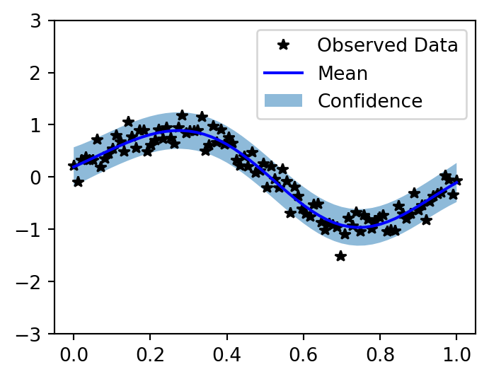

Question 4.1: Different Kernel

Using the code above, try a different kernel from the docs and plot the results. Doesn’t matter if it is better or worse, but you should try to pick a kernel that has different parameters to fit.

class ExactGPModelMatern(gpytorch.models.ExactGP):
    def __init__(
        self, train_x, train_y, likelihood
    ):
        super().__init__(
            train_x, train_y, likelihood
        )
        self.mean_module = (
            gpytorch.means.ConstantMean()
        )
        self.covar_module = (
            gpytorch.kernels.ScaleKernel(
                gpytorch.kernels.MaternKernel(
                    nu=1.5
                )
            )
        )

    def forward(self, x):
        mean_x = self.mean_module(x)
        covar_x = self.covar_module(x)
        return (
            gpytorch.distributions
            .MultivariateNormal(mean_x, covar_x)
        )

likelihood_m = (
    gpytorch.likelihoods.GaussianLikelihood()
)
model_m = ExactGPModelMatern(
    train_x, train_y, likelihood_m
)
model_m.train()
likelihood_m.train()

optimizer_m = torch.optim.Adam(
    model_m.parameters(), lr=0.1
)
mll_m = (
    gpytorch.mlls.ExactMarginalLogLikelihood(
        likelihood_m, model_m
    )
)

for i in range(50):
    optimizer_m.zero_grad()
    output = model_m(train_x)
    loss = -mll_m(output, train_y)
    loss.backward()
    if (i + 1) % 10 == 0:
        ls = (
            model_m.covar_module
            .base_kernel.lengthscale.item()
        )
        ns = model_m.likelihood.noise.item()
        print(
            f"Iter {i+1}/50"
            f" - Loss: {loss.item():.3f}"
            f"   lengthscale: {ls:.3f}"
            f"   noise: {ns:.3f}"
        )
    optimizer_m.step()

model_m.eval()
likelihood_m.eval()

with (
    torch.no_grad(),
    gpytorch.settings.fast_pred_var(),
):
    test_x = torch.linspace(0, 1, 51)
    observed_pred_m = likelihood_m(
        model_m(test_x)
    )

with torch.no_grad():
    f, ax = plt.subplots(1, 1, figsize=(4, 3))
    lower, upper = (
        observed_pred_m.confidence_region()
    )
    ax.plot(
        train_x.numpy(), train_y.numpy(), 'k*'
    )
    ax.plot(
        test_x.numpy(),
        observed_pred_m.mean.numpy(), 'b',
    )
    ax.fill_between(
        test_x.numpy(),
        lower.numpy(), upper.numpy(),
        alpha=0.5,
    )
    ax.set_ylim([-3, 3])
    ax.legend(
        ['Observed Data', 'Mean', 'Confidence']
    )
    ax.set_title(
        'GP with Matern(nu=1.5) Kernel'
    )

Iter 10/50 - Loss: 0.546   lengthscale: 0.371   noise: 0.340
Iter 20/50 - Loss: 0.181   lengthscale: 0.390   noise: 0.137
Iter 30/50 - Loss: -0.106   lengthscale: 0.384   noise: 0.054
Iter 40/50 - Loss: -0.196   lengthscale: 0.370   noise: 0.025
Iter 50/50 - Loss: -0.179   lengthscale: 0.356   noise: 0.020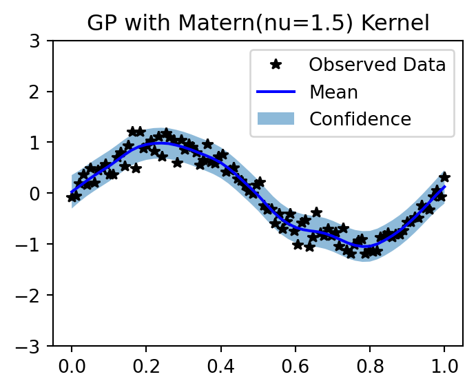

The Matern kernel with \(\nu = 1.5\) produces slightly less smooth predictions than the RBF kernel, since the RBF corresponds to \(\nu \to \infty\).

Question 4.2 (BONUS): Noiseless GP Interpolation

Now take the code above:

1. Remove the noise in the DGP
2. Decrease the number of generated datapoints to maybe 10 or so.
3. Try to see how to fit a GP without any observational noise, so that it interpolates the data. This may require changing the likelihood object in the loop above.

N_pts = 10
train_x_small = torch.linspace(0, 1, N_pts)
train_y_small = torch.sin(
    train_x_small * (2 * math.pi)
)  # no noise

# Relaxed noise constraint for near-zero noise
likelihood_noiseless = (
    gpytorch.likelihoods.GaussianLikelihood(
        noise_constraint=(
            gpytorch.constraints.GreaterThan(
                1e-8
            )
        )
    )
)
# very small noise for numerical stability
likelihood_noiseless.noise = 1e-6
# Freeze noise so optimizer doesn't change it
likelihood_noiseless.noise_covar.raw_noise.requires_grad = False

model_noiseless = ExactGPModel(
    train_x_small,
    train_y_small,
    likelihood_noiseless,
)
model_noiseless.train()
likelihood_noiseless.train()

optimizer_nl = torch.optim.Adam(
    model_noiseless.parameters(), lr=0.1
)
mll_nl = (
    gpytorch.mlls.ExactMarginalLogLikelihood(
        likelihood_noiseless, model_noiseless
    )
)

for i in range(100):
    optimizer_nl.zero_grad()
    output = model_noiseless(train_x_small)
    loss = -mll_nl(output, train_y_small)
    loss.backward()
    optimizer_nl.step()

model_noiseless.eval()
likelihood_noiseless.eval()

with (
    torch.no_grad(),
    gpytorch.settings.fast_pred_var(),
):
    test_x = torch.linspace(0, 1, 200)
    observed_pred_nl = likelihood_noiseless(
        model_noiseless(test_x)
    )

with torch.no_grad():
    f, ax = plt.subplots(1, 1, figsize=(6, 4))
    lower, upper = (
        observed_pred_nl.confidence_region()
    )
    ax.plot(
        train_x_small.numpy(),
        train_y_small.numpy(),
        'k*', markersize=10,
    )
    ax.plot(
        test_x.numpy(),
        observed_pred_nl.mean.numpy(), 'b',
    )
    ax.fill_between(
        test_x.numpy(),
        lower.numpy(), upper.numpy(),
        alpha=0.5,
    )
    true_fn = torch.sin(
        test_x * 2 * math.pi
    ).numpy()
    ax.plot(
        test_x.numpy(), true_fn,
        'r--', alpha=0.5,
        label='True function',
    )
    ax.set_ylim([-3, 3])
    ax.legend(
        ['Observations', 'GP Mean',
         'Confidence', 'True function']
    )
    ax.set_title(
        'Noiseless GP Interpolation (N=10)'
    )

/home/runner/work/grad_econ_ML/grad_econ_ML/.venv/lib/python3.13/site-packages/gpytorch/distributions/multivariate_normal.py:375: NumericalWarning: Negative variance values detected. This is likely due to numerical instabilities. Rounding negative variances up to 1e-06.
  warnings.warn(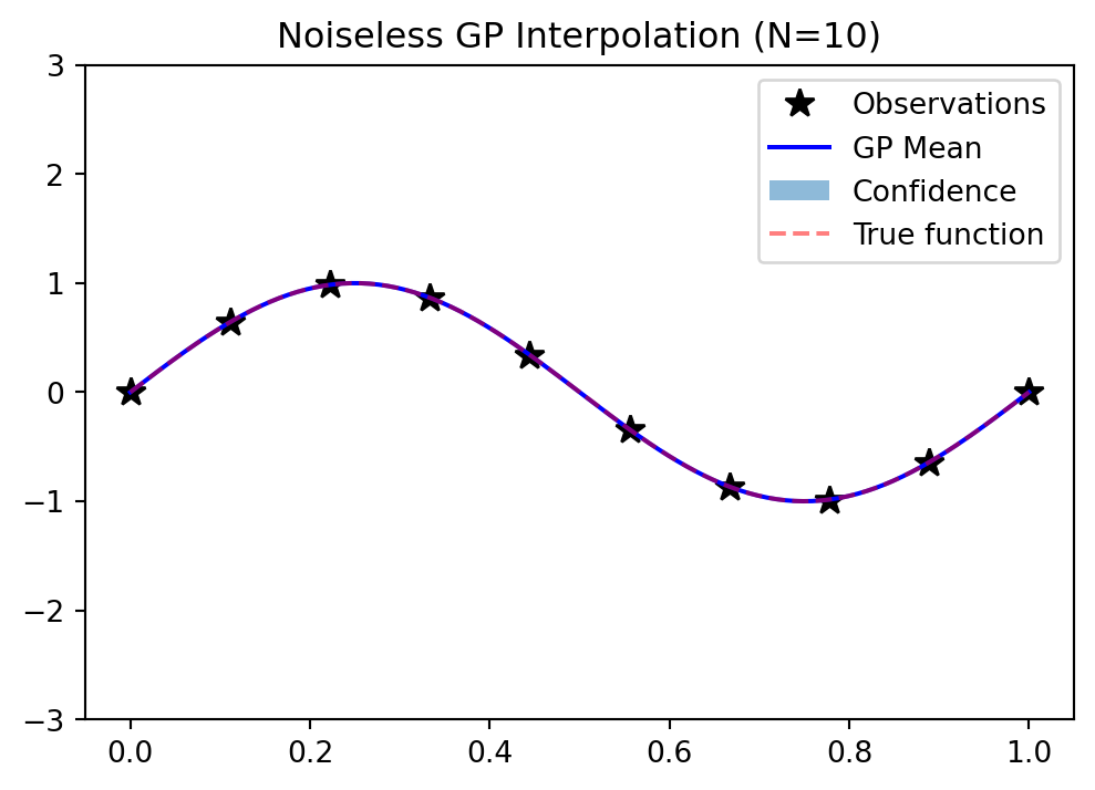

The key insight is constraining the likelihood noise to a very small value so the GP interpolates (passes through) the training points rather than smoothing over them.

Question 5: OpenAI API

Setting up OpenAI to access ChatGPT and embeddings programmatically.

Question 5.1: Setup and First Call

Setup an account on the OpenAI platform:

• Sign up
• Go to the API keys tab and create a key
• In your terminal, set OPENAI_API_KEY to this value (see here)

Given the change in the environment variable, you may need to restart your browser/editor/etc.

Get the following code running, which shows a prompt:

client = OpenAI()
response = client.responses.create(
    model="gpt-4o-mini",
    temperature=0.7,
    instructions=(
        "You are generating numbers"
        " that are easy to parse."
    ),
    input="Give me a list of 3 numbers",
)
print(response.output_text)

This is a setup step — just run the code above after setting the OPENAI_API_KEY environment variable. If it prints a list of numbers, you’re done.

Question 5.2: Temperature Exploration

Take that prompt and run it a bunch of times with temperature = 0.0. What happens and why?

Next, run it a bunch of times with temperature = 2.0, which is the maximum allowed by the API. What happens and why?

client = OpenAI()

print("=== temperature = 0.0 (deterministic) ===")
for i in range(3):
    response = client.responses.create(
        model="gpt-4o-mini",
        temperature=0.0,
        instructions=(
            "You are generating numbers"
            " that are easy to parse."
        ),
        input="Give me a list of 3 numbers",
    )
    print(
        f"  Run {i+1}: {response.output_text}"
    )

print("\n=== temperature = 2.0 (max allowed) ===")
for i in range(3):
    response = client.responses.create(
        model="gpt-4o-mini",
        temperature=2.0,
        instructions=(
            "You are generating numbers"
            " that are easy to parse."
        ),
        input="Give me a list of 3 numbers",
    )
    print(
        f"  Run {i+1}: {response.output_text}"
    )

Explanation: With temperature = 0.0, the model always picks the highest-probability token at each step, so the output is nearly deterministic — you get the same (or very similar) list each time. With temperature = 2.0, the softmax distribution is flattened dramatically, making low-probability tokens much more likely. The output becomes erratic and sometimes incoherent, as the model samples from an almost-uniform distribution over the vocabulary.

Question 5.3: Parsing LLM Output

Modify the instructions in that prompt until you can easily parse the response.output_text into a list, reliably, with temperature = 0.7.

client = OpenAI()
response = client.responses.create(
    model="gpt-4o-mini",
    temperature=0.7,
    instructions=(  # modify this
        "You are generating numbers"
        " that are easy to parse."
    ),
    input="Give me a list of 3 numbers",
)
print(response.output_text)
# Add parsing logic

import json

client = OpenAI()
response = client.responses.create(
    model="gpt-4o-mini",
    temperature=0.7,
    instructions=(
        "You must respond with ONLY"
        " a JSON array of numbers."
        " No text, no explanation,"
        " just the JSON array."
        " Example: [1, 2, 3]"
    ),
    input="Give me a list of 3 numbers",
    text={
        "format": {"type": "json_object"}
    },
)
raw = response.output_text
print(f"Raw output: {raw}")
numbers = json.loads(raw)
print(f"Parsed list: {numbers}")
print(
    f"Type: {type(numbers)},"
    f" Length: {len(numbers)}"
)

The Responses API supports structured output via text={"format": {"type": "json_object"}}, which guarantees valid JSON. Combined with clear instructions, json.loads() reliably parses the response.