import numpy as np
import matplotlib.pyplot as plt
import jax
import jax.numpy as jnp
from jax import grad, jvp, vjp
from jax import random
from numpy.linalg import condECON622: Problem Set 3
Packages
Add whatever packages you wish here
Question 1: Conditioning and Preconditioned Gradient Descent
In this question, you will explore how the condition number affects gradient descent convergence and implement a simple diagonal preconditioner to improve performance.
We consider minimizing the quadratic function:
\[ f(x) = \frac{1}{2} x^\top P x \]
where \(P\) is a symmetric positive definite matrix. The gradient is \(\nabla f(x) = P x\), so the minimum is at \(x^* = 0\).
Starter Code
The following function visualizes gradient descent on a 2D quadratic:
def plot_gd_steps(N_steps, x_0, Lambda, eta, theta=np.pi/6):
    """
    Plot gradient descent steps on a 2D quadratic f(x) = 0.5 * x^T P x
    where P = Q @ diag(Lambda) @ Q^T for rotation angle theta.

    Args:
        N_steps: Number of GD iterations to plot
        x_0: Initial point [x1, x2]
        Lambda: Eigenvalues [lambda1, lambda2] (condition number = max/min)
        eta: Step size (learning rate)
        theta: Rotation angle for Q (default: pi/6)
    """
    c, s = np.cos(theta), np.sin(theta)
    Q = np.array([[c, -s], [s, c]])
    P = Q @ np.diag(Lambda) @ Q.T
    gd_step = lambda x: x - eta * P @ x

    x_vals = np.linspace(-1, 1, 100)
    X1, X2 = np.meshgrid(x_vals, x_vals)
    Z = 0.5 * (P[0,0]*X1**2 + 2*P[0,1]*X1*X2 + P[1,1]*X2**2)

    plt.figure(figsize=(6, 5))
    plt.contour(X1, X2, Z, levels=20, cmap='viridis')

    x_current = np.array(x_0)
    for i in range(N_steps):
        x_next = gd_step(x_current)
        plt.arrow(x_current[0], x_current[1],
                  x_next[0] - x_current[0], x_next[1] - x_current[1],
                  head_width=0.03, head_length=0.02, fc='red', ec='red')
        x_current = x_next

    plt.xlabel('x1'); plt.ylabel('x2')
    plt.gca().set_aspect('equal')
    return plt.gcf()
Question 1.1: Explore Conditioning Visually
Run the visualization with different condition numbers and observe how the contours change shape.
x_0 = [0.9, 0.0]
eta = 0.5

# Well-conditioned: kappa = 2
Lambda_good = np.array([1.0, 0.5])
plot_gd_steps(5, x_0, Lambda_good, eta)
plt.title(r'$\kappa = 2$: Well-conditioned')
plt.show()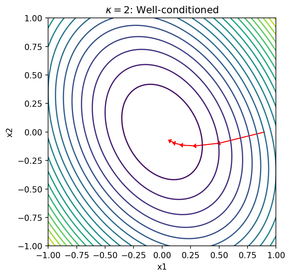
Now run with \(\kappa = 10\) (eigenvalues [1.0, 0.1]) and \(\kappa = 100\) (eigenvalues [1.0, 0.01]).
# modify here(double click to edit your answer)
Explain in 2-3 sentences why gradient descent struggles with poorly-conditioned problems (narrow ellipses).
# SOLUTIONS
# kappa = 10
Lambda_10 = np.array([1.0, 0.1])
plot_gd_steps(5, x_0, Lambda_10, eta)
plt.title(r'$\kappa = 10$: Moderately conditioned')
plt.show()

# kappa = 100
Lambda_100 = np.array([1.0, 0.01])
plot_gd_steps(5, x_0, Lambda_100, eta)
plt.title(r'$\kappa = 100$: Poorly conditioned')
plt.show()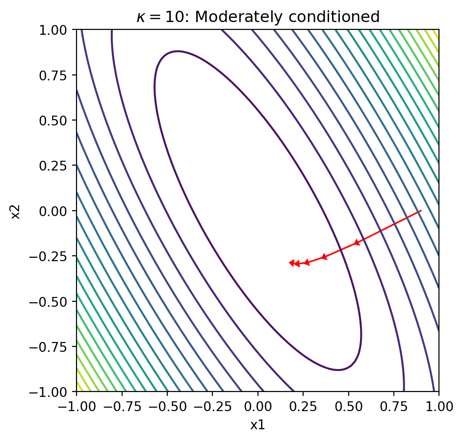
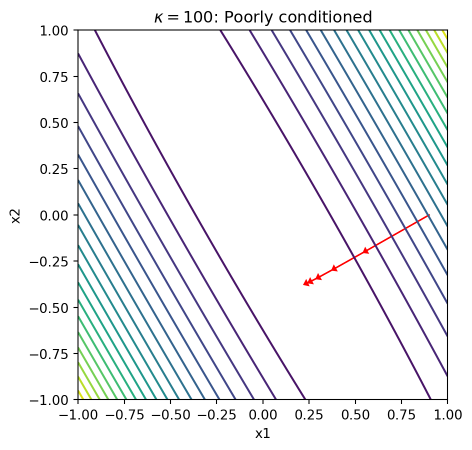
Explanation: When the condition number is large, the contours form narrow ellipses. The gradient points perpendicular to these contours, which means it points mostly in the “short” direction of the ellipse rather than toward the minimum. This causes gradient descent to zigzag slowly along the narrow valley, requiring many iterations to converge.
Question 1.2: Count Iterations to Convergence
Use the following function to count how many iterations GD needs to converge:
def count_gd_iterations(x_0, P, eta, tol=1e-6, max_iter=5000):
    """Count iterations until ||x|| < tol"""
    x = np.array(x_0)
    for i in range(max_iter):
        if np.linalg.norm(x) < tol:
            return i
        x = x - eta * P @ x
    return max_iter  # didn't converge
Helper function to create \(P\) from eigenvalues:
def make_P(Lambda, theta=np.pi/6):
    """Create P = Q @ diag(Lambda) @ Q^T with rotation angle theta"""
    c, s = np.cos(theta), np.sin(theta)
    Q = np.array([[c, -s], [s, c]])
    return Q @ np.diag(Lambda) @ Q.T
Count iterations for \(\kappa = 2, 10, 100\) with eta = 0.5 and x_0 = [0.9, 0.0]:
# modify here(double click to edit your answer)
Report the iteration counts and explain the relationship between \(\kappa\) and convergence rate.
# SOLUTIONS
x_0 = [0.9, 0.0]
eta = 0.5

for kappa in [2, 10, 100]:
    Lambda = np.array([1.0, 1.0/kappa])
    P = make_P(Lambda)
    iters = count_gd_iterations(x_0, P, eta)
    print(f"kappa = {kappa}: {iters} iterations")
kappa = 2: 46 iterations
kappa = 10: 254 iterations
kappa = 100: 2597 iterationsExplanation: The iteration count grows roughly linearly with \(\kappa\). Theory tells us that gradient descent converges at rate \(O((1 - 1/\kappa)^k)\), so the number of iterations to reach tolerance \(\epsilon\) is \(O(\kappa \log(1/\epsilon))\). Doubling the condition number roughly doubles the iterations needed.
Question 1.3 (BONUS): Understand Preconditioned Gradient Descent
Standard gradient descent updates:
\[ x^{k+1} = x^k - \eta \nabla f(x^k) = x^k - \eta P x^k \]
Preconditioned gradient descent scales the gradient by a matrix \(D^{-1}\):
\[ x^{k+1} = x^k - \eta D^{-1} \nabla f(x^k) = x^k - \eta D^{-1} P x^k \]
Your task: Show that preconditioned GD is equivalent to standard GD on a transformed problem.
Let \(\tilde{x} = D^{1/2} x\) (assuming \(D\) is diagonal with positive entries). Show that:
- The objective becomes \(\tilde{f}(\tilde{x}) = \frac{1}{2} \tilde{x}^\top \tilde{P} \tilde{x}\) where \(\tilde{P} = D^{-1/2} P D^{-1/2}\)
- If we choose \(D = \text{diag}(P)\), what are the diagonal entries of \(\tilde{P}\)?
(double click to edit your answer)
Derivation:
Part 1: Let \(\tilde{x} = D^{1/2} x\), so \(x = D^{-1/2} \tilde{x}\).
Substituting into \(f(x) = \frac{1}{2} x^\top P x\):
\[ \tilde{f}(\tilde{x}) = \frac{1}{2} (D^{-1/2} \tilde{x})^\top P (D^{-1/2} \tilde{x}) = \frac{1}{2} \tilde{x}^\top D^{-1/2} P D^{-1/2} \tilde{x} = \frac{1}{2} \tilde{x}^\top \tilde{P} \tilde{x} \]
where \(\tilde{P} = D^{-1/2} P D^{-1/2}\).
Part 2: If \(D = \text{diag}(P)\), then \(D_{ii} = P_{ii}\).
The diagonal entries of \(\tilde{P}\) are:
\[ \tilde{P}_{ii} = \frac{P_{ii}}{\sqrt{D_{ii}} \sqrt{D_{ii}}} = \frac{P_{ii}}{P_{ii}} = 1 \]
So \(\tilde{P}\) has all 1’s on the diagonal! This tends to improve the condition number because it “normalizes” the scale of each coordinate.
Question 1.4: Implement Diagonal Preconditioning
Implement preconditioned GD and compare iteration counts:
def count_preconditioned_gd_iterations(x_0, P, D_inv, eta, tol=1e-6, max_iter=5000):
    """Count iterations for preconditioned GD: x_{k+1} = x_k - eta * D^{-1} @ P @ x_k"""
    x = np.array(x_0)
    for i in range(max_iter):
        if np.linalg.norm(x) < tol:
            return i
        # modify here: implement preconditioned step
        x = x - eta * P @ x
    return max_iter
Test with \(\kappa = 100\):
Lambda = np.array([1.0, 0.01])
P = make_P(Lambda)
D_inv = np.diag(1.0 / np.diag(P))  # D^{-1} where D = diag(P)

# modify here: compare iterations with and without preconditioning
# SOLUTIONS
def count_preconditioned_gd_iterations(x_0, P, D_inv, eta, tol=1e-6, max_iter=5000):
"""Count iterations for preconditioned GD: x_{k+1} = x_k - eta * D^{-1} @ P @ x_k"""
x = np.array(x_0)
for i in range(max_iter):
if np.linalg.norm(x) < tol:
return i
grad = P @ x
x = x - eta * D_inv @ grad
return max_iter
Lambda = np.array([1.0, 0.01])
P = make_P(Lambda)
D_inv = np.diag(1.0 / np.diag(P))
x_0 = [0.9, 0.0]
eta = 0.5
iters_no_precond = count_gd_iterations(x_0, P, eta)
iters_precond = count_preconditioned_gd_iterations(x_0, P, D_inv, eta)
print(f"Without preconditioning: {iters_no_precond} iterations")
print(f"With preconditioning: {iters_precond} iterations")
print(f"Speedup: {iters_no_precond / iters_precond:.1f}x")Without preconditioning: 2597 iterations
With preconditioning: 1042 iterations
Speedup: 2.5xQuestion 1.5: Verify the Condition Number Improvement
Compute and compare the condition numbers before and after preconditioning:
Lambda = np.array([1.0, 0.01])
P = make_P(Lambda)
D = np.diag(np.diag(P))
D_sqrt_inv = np.diag(1.0 / np.sqrt(np.diag(P)))

# Preconditioned matrix: D^{-1/2} P D^{-1/2}
P_precond = D_sqrt_inv @ P @ D_sqrt_inv

# modify here: compute and print condition numbers
print(f"cond(P) = ...")
print(f"cond(P_precond) = ...")
cond(P) = ...
cond(P_precond) = ...(double click to edit your answer)
Explain why the diagonal preconditioner improves the condition number for this problem.
# SOLUTIONS
print(f"cond(P) = {cond(P):.2f}")
print(f"cond(P_precond) = {cond(P_precond):.2f}")
print(f"Diagonal of P_precond: {np.diag(P_precond)}")
cond(P) = 100.00
cond(P_precond) = 75.49
Diagonal of P_precond: [1. 1.]Explanation: The diagonal preconditioner sets all diagonal entries of \(\tilde{P}\) to 1, which removes the dominant source of poor conditioning in many problems. In this 2D example with rotated axes, the improvement is dramatic because the diagonal captures much of the eigenvalue spread. In general, diagonal preconditioning works best when the matrix is close to diagonal-dominant.
Question 1.6: When Diagonal Preconditioning Fails
The effectiveness of diagonal preconditioning depends on the rotation angle \(\theta\) used to construct \(P = Q(\theta) \Lambda Q(\theta)^\top\).
Repeat the preconditioning experiment from Q1.4-1.5 with \(\theta = \pi/4\) (a 45-degree rotation). Compare iteration counts with and without preconditioning, and compute the condition numbers of \(P\) and \(\tilde{P}\).
Lambda = np.array([1.0, 0.01])

# modify here: construct P with theta = pi/4, compute D_inv, and compare
# iterations with and without preconditioning
# Also compute cond(P) and cond(P_precond)
(double click to edit your answer)
- What do you observe about the iteration counts?
- Examine the diagonal entries of \(P\) at \(\theta = \pi/4\). Why does diagonal preconditioning fail here?
- What is \(D^{-1}\) in this case, and what does the preconditioned step \(x - \eta D^{-1} P x\) simplify to?
# SOLUTIONS
Lambda = np.array([1.0, 0.01])
theta_45 = np.pi / 4
P_45 = make_P(Lambda, theta=theta_45)
D_inv_45 = np.diag(1.0 / np.diag(P_45))

x_0 = [0.9, 0.0]
eta = 0.5

iters_no_precond = count_gd_iterations(x_0, P_45, eta)
iters_precond = count_preconditioned_gd_iterations(x_0, P_45, D_inv_45, eta)

print(f"theta = pi/4 (45-degree rotation)")
print(f"Without preconditioning: {iters_no_precond} iterations")
print(f"With preconditioning: {iters_precond} iterations")
print(f"Speedup: {iters_no_precond / max(iters_precond, 1):.1f}x")

print(f"\nDiagonal entries of P: P[0,0] = {P_45[0,0]:.4f}, P[1,1] = {P_45[1,1]:.4f}")

D_sqrt_inv_45 = np.diag(1.0 / np.sqrt(np.diag(P_45)))
P_precond_45 = D_sqrt_inv_45 @ P_45 @ D_sqrt_inv_45
print(f"\ncond(P) = {cond(P_45):.2f}")
print(f"cond(P_precond) = {cond(P_precond_45):.2f}")
theta = pi/4 (45-degree rotation)
Without preconditioning: 2667 iterations
With preconditioning: 1344 iterations
Speedup: 2.0x
Diagonal entries of P: P[0,0] = 0.5050, P[1,1] = 0.5050
cond(P) = 100.00
cond(P_precond) = 100.00Explanation:
At \(\theta = \pi/4\), the diagonal entries of \(P\) are:
\[ P_{00} = \cos^2(\pi/4)\,\lambda_1 + \sin^2(\pi/4)\,\lambda_2 = \frac{\lambda_1 + \lambda_2}{2} \]
\[ P_{11} = \sin^2(\pi/4)\,\lambda_1 + \cos^2(\pi/4)\,\lambda_2 = \frac{\lambda_1 + \lambda_2}{2} \]
Since \(P_{00} = P_{11}\), the diagonal preconditioner \(D = \text{diag}(P)\) is a scalar multiple of the identity: \(D = \frac{\lambda_1 + \lambda_2}{2} I\). Therefore \(D^{-1} = \frac{2}{\lambda_1 + \lambda_2} I\), and the preconditioned step becomes:
\[ x - \eta D^{-1} P x = x - \frac{2\eta}{\lambda_1 + \lambda_2} P x \]
This is just standard gradient descent with a rescaled step size \(\eta' = \frac{2\eta}{\lambda_1 + \lambda_2}\). The condition number is unchanged: \(\kappa(\tilde{P}) = \kappa(P)\).
Note: The iteration counts may still differ because \(D^{-1}\) changes the effective step size (here \(\eta' \approx 2 \times 0.5 / 1.01 \approx 0.99\) vs \(\eta = 0.5\)). But this is not a preconditioning improvement — it is just step-size tuning. The convergence rate (governed by \(\kappa\)) is identical.
Lesson: Diagonal preconditioning fails when all diagonal entries of \(P\) are equal, which happens at \(\theta = \pi/4\) because the rotation symmetrically mixes the eigenvalues. More generally, diagonal preconditioning is ineffective when the poor conditioning comes from off-diagonal structure rather than diagonal scaling differences.
Question 2: Vectorized AD Rule for Matrix-Vector Product
In this question, you will derive the JVP and VJP rules for a vectorized operation (matrix-vector multiplication) and verify your implementation against JAX.
Consider the function \(f(A, x) = Ax\) where \(A \in \mathbb{R}^{m \times n}\) and \(x \in \mathbb{R}^n\).
Question 2.1: Derive the JVP Rule
Given tangents \(\dot{A} \in \mathbb{R}^{m \times n}\) and \(\dot{x} \in \mathbb{R}^n\), derive the pushforward (JVP):
\[ \dot{y} = \partial f(A, x)[(\dot{A}, \dot{x})] = ? \]
Hint: Use the product rule for differentiation.
(double click to edit your answer)
Derivation:
Using the product rule:
\[ \dot{y} = \frac{d}{dt}\bigg|_{t=0} (A + t\dot{A})(x + t\dot{x}) = \dot{A} x + A \dot{x} \]
So the JVP rule is: \(\dot{y} = \dot{A} x + A \dot{x}\)
Question 2.2 (BONUS): Derive the VJP Rule
Given a cotangent \(\bar{y} \in \mathbb{R}^m\), derive the pullback (VJP):
\[ (\bar{A}, \bar{x}) = \partial f(A, x)^\top[\bar{y}] = ? \]
Hint for adjoint algebra: Start with the inner product \(\langle \bar{y}, \dot{y} \rangle = \langle \bar{y}, \dot{A} x + A \dot{x} \rangle\) and rearrange to identify \(\bar{A}\) and \(\bar{x}\).
Recall that for matrices, \(\langle U, V \rangle = \text{Tr}(U^\top V)\), and for vectors, \(\langle u, v \rangle = u^\top v\).
(double click to edit your answer)
Derivation:
We need to find \(\bar{A}\) and \(\bar{x}\) such that:
\[ \langle (\bar{A}, \bar{x}), (\dot{A}, \dot{x}) \rangle = \langle \bar{y}, \dot{y} \rangle \]
Expanding the right side:
\[ \langle \bar{y}, \dot{A} x + A \dot{x} \rangle = \langle \bar{y}, \dot{A} x \rangle + \langle \bar{y}, A \dot{x} \rangle \]
For the first term, using trace properties:
\[ \langle \bar{y}, \dot{A} x \rangle = \bar{y}^\top (\dot{A} x) = \text{Tr}(\bar{y}^\top \dot{A} x) = \text{Tr}(x \bar{y}^\top \dot{A}) = \langle \bar{y} x^\top, \dot{A} \rangle \]
So \(\bar{A} = \bar{y} x^\top\) (the outer product).
For the second term:
\[ \langle \bar{y}, A \dot{x} \rangle = \bar{y}^\top A \dot{x} = (A^\top \bar{y})^\top \dot{x} = \langle A^\top \bar{y}, \dot{x} \rangle \]
So \(\bar{x} = A^\top \bar{y}\).
Summary: \(\bar{A} = \bar{y} x^\top\) and \(\bar{x} = A^\top \bar{y}\)
Question 2.3: Implement and Verify JVP
Implement your JVP rule and verify against JAX:
def matvec(A, x):
    """f(A, x) = A @ x"""
    return A @ x

def matvec_jvp(A, x, A_dot, x_dot):
    """Your implementation of the JVP rule: returns y_dot"""
    # modify here
    pass

# Test data
key = random.PRNGKey(42)
keys = random.split(key, 4)
m, n = 4, 3
A = random.normal(keys[0], (m, n))
x = random.normal(keys[1], (n,))
A_dot = random.normal(keys[2], (m, n))
x_dot = random.normal(keys[3], (n,))

# modify here: compare to JAX jvp
# SOLUTIONS
def matvec_jvp(A, x, A_dot, x_dot):
"""JVP rule: y_dot = A_dot @ x + A @ x_dot"""
return A_dot @ x + A @ x_dot
# Compare to JAX
primals = (A, x)
tangents = (A_dot, x_dot)
y, y_dot_jax = jvp(matvec, primals, tangents)
y_dot_manual = matvec_jvp(A, x, A_dot, x_dot)
print(f"JAX JVP result: {y_dot_jax}")
print(f"Manual JVP result: {y_dot_manual}")
print(f"Match: {jnp.allclose(y_dot_manual, y_dot_jax)}")JAX JVP result: [ 0.30276608 0.11958396 2.7425175 -0.5717054 ]
Manual JVP result: [ 0.30276608 0.11958396 2.7425175 -0.5717054 ]
Match: TrueQuestion 2.4: Implement and Verify VJP
Implement your VJP rule and verify against JAX:
def matvec_vjp(A, x, y_bar):
    """Your implementation of the VJP rule: returns (A_bar, x_bar)"""
    # modify here
    pass

# Test cotangent
y_bar = random.normal(random.PRNGKey(99), (m,))

# modify here: compare to JAX vjp
# SOLUTIONS
def matvec_vjp(A, x, y_bar):
"""VJP rule: A_bar = y_bar @ x^T (outer product), x_bar = A^T @ y_bar"""
A_bar = jnp.outer(y_bar, x)
x_bar = A.T @ y_bar
return A_bar, x_bar
# Compare to JAX
y, vjp_fun = vjp(matvec, A, x)
A_bar_jax, x_bar_jax = vjp_fun(y_bar)
A_bar_manual, x_bar_manual = matvec_vjp(A, x, y_bar)
print(f"A_bar match: {jnp.allclose(A_bar_manual, A_bar_jax)}")
print(f"x_bar match: {jnp.allclose(x_bar_manual, x_bar_jax)}")
print(f"\nJAX x_bar: {x_bar_jax}")
print(f"Manual x_bar (A^T @ y_bar): {x_bar_manual}")A_bar match: True
x_bar match: True
JAX x_bar: [0.02138905 0.06485057 3.1164155 ]
Manual x_bar (A^T @ y_bar): [0.02138905 0.06485057 3.1164155 ](double click to edit your answer)
Explain in 2-3 sentences the connection between the VJP formula \(\bar{x} = A^\top \bar{y}\) and the “adjoint” or “transpose” terminology used in automatic differentiation.
The VJP is called the “adjoint” or “pullback” because it literally involves the transpose (adjoint) of the Jacobian. For a linear function \(f(x) = Ax\), the Jacobian is just \(A\) itself. The VJP computes \(J^\top \bar{y} = A^\top \bar{y}\), which is exactly the matrix transpose applied to the cotangent vector. This is why reverse-mode AD is sometimes called “adjoint mode” - it propagates gradients backward through the computational graph using transposes at each step.
Question 3 (BONUS): Sensitivity Analysis via the LLS Adjoint
In this question, you will derive and apply the VJP (adjoint) rule for linear least squares to perform sensitivity analysis: understanding how each observation affects the estimated coefficients.
The Linear Least Squares Problem
Given design matrix \(X \in \mathbb{R}^{n \times p}\) and observations \(y \in \mathbb{R}^n\), the least squares solution is:
\[ \hat{\beta} = (X^\top X)^{-1} X^\top y \]
Question 3.1: The LLS Adjoint Rule
The VJP rule for \(\hat{\beta} = \text{LLS}(X, y)\) is derived by chaining through the matrix inverse and products.
Given: A cotangent \(\bar{\beta} \in \mathbb{R}^p\) (representing “how much we care about each coefficient”)
Compute:
- Solve the linear system: \(g = (X^\top X)^{-1} \bar{\beta}\)
- Compute the residual: \(r = y - X\hat{\beta}\)
Then the adjoints are:
\[ \bar{y} = X g \]
\[ \bar{X} = r\, g^\top - (Xg)\, \hat{\beta}^\top \]
(double click to edit your answer)
Explain in 2-3 sentences why this is computationally powerful: if we want to know how \(\hat{\beta}_0\) depends on ALL \(n\) observations \(y_i\), how many backward passes do we need?
We only need one backward pass! By setting \(\bar{\beta} = e_0 = [1, 0, 0, \ldots]\), we get \(\bar{y} = Xg\) which gives us \(\partial \hat{\beta}_0 / \partial y_i\) for ALL \(i = 1, \ldots, n\) simultaneously. This is \(O(n)\) work vs \(O(n^2)\) if we computed each sensitivity separately via finite differences.
Question 3.2: Generate Data and Compute LLS
# Generate random regression data
key = random.PRNGKey(123)
keys = random.split(key, 3)

n = 1000  # observations
p = 3     # parameters

# True coefficients
beta_true = jnp.array([2.0, -1.0, 0.5])

# Random design matrix and noisy observations
X = random.normal(keys[0], (n, p))
noise = 0.1 * random.normal(keys[1], (n,))
y = X @ beta_true + noise

# Compute LLS solution
beta_hat = jnp.linalg.lstsq(X, y)[0]
print(f"True beta: {beta_true}")
print(f"Estimated beta: {beta_hat}")
True beta: [ 2. -1. 0.5]
Estimated beta: [ 2.0004642 -1.0009896 0.49019286]Question 3.3: Manual Sensitivity Calculation
Use the LLS adjoint rule to compute \(\partial \hat{\beta}_0 / \partial y_i\) for all observations.
# We want sensitivity of beta_hat[0] to each y_i
# Set beta_bar = e_0 = [1, 0, 0]
beta_bar = jnp.array([1.0, 0.0, 0.0])

# modify here: compute g, r, and y_bar using the adjoint formula
# g = (X^T X)^{-1} @ beta_bar
# r = y - X @ beta_hat
# y_bar = X @ g
# SOLUTIONS
# Step 1: Solve (X^T X) g = beta_bar
XtX = X.T @ X
g = jnp.linalg.solve(XtX, beta_bar)
# Step 2: Compute residual (not needed for y_bar, but useful for X_bar)
r = y - X @ beta_hat
# Step 3: Compute y_bar = X @ g
y_bar_manual = X @ g
print(f"Shape of y_bar: {y_bar_manual.shape}")
print(f"First 10 sensitivities: {y_bar_manual[:10]}")
print(f"Sum of sensitivities: {y_bar_manual.sum():.6f}")Shape of y_bar: (1000,)
First 10 sensitivities: [-0.00044072 -0.00028137 -0.0006584 0.00223566 -0.00035178 0.00081971
-0.00016767 -0.00067485 0.00156292 0.00026478]
Sum of sensitivities: 0.000539Question 3.4: Verify with JAX VJP
Use JAX’s built-in autodiff to verify your manual calculation:
def lls(y):
    """LLS as a function of y only (X is fixed)"""
    return jnp.linalg.lstsq(X, y)[0]

# modify here: use vjp to compute sensitivity of beta_hat[0] to y
# beta_hat_jax, vjp_fun = vjp(lls, y)
# y_bar_jax, = vjp_fun(beta_bar)
# Compare to y_bar_manual
# SOLUTIONS
beta_hat_jax, vjp_fun = vjp(lls, y)
y_bar_jax, = vjp_fun(beta_bar)
print(f"Manual y_bar[:5]: {y_bar_manual[:5]}")
print(f"JAX y_bar[:5]: {y_bar_jax[:5]}")
print(f"Match: {jnp.allclose(y_bar_manual, y_bar_jax)}")Manual y_bar[:5]: [-0.00044072 -0.00028137 -0.0006584 0.00223566 -0.00035178]
JAX y_bar[:5]: [-0.00044072 -0.00028137 -0.0006584 0.00223566 -0.00035178]
Match: TrueQuestion 3.5: Interpret the Sensitivities
Plot the sensitivities and identify influential observations:
# modify here: create a plot showing the sensitivities
# plt.figure(figsize=(10, 4))
# plt.plot(y_bar_manual, 'o', alpha=0.5, markersize=3)
# plt.xlabel('Observation index i')
# plt.ylabel(r'$\partial \hat{\beta}_0 / \partial y_i$')
# plt.title('Sensitivity of $\\hat{\\beta}_0$ to each observation')
# plt.show()

# Find the most influential observations
# top_indices = jnp.argsort(jnp.abs(y_bar_manual))[-5:]
(double click to edit your answer)
- What determines whether an observation has high sensitivity (large \(|\partial \hat{\beta}_0 / \partial y_i|\))?
- How does this relate to the concept of “leverage” in regression diagnostics?
# SOLUTIONS
plt.figure(figsize=(10, 4))
plt.plot(y_bar_manual, 'o', alpha=0.5, markersize=3)
plt.xlabel('Observation index i')
plt.ylabel(r'$\partial \hat{\beta}_0 / \partial y_i$')
plt.title('Sensitivity of $\\hat{\\beta}_0$ to each observation')
plt.axhline(y=0, color='k', linestyle='--', alpha=0.3)
plt.show()

# Find most influential observations
top_indices = jnp.argsort(jnp.abs(y_bar_manual))[-5:]
print(f"Most influential observation indices: {top_indices}")
print(f"Their sensitivities: {y_bar_manual[top_indices]}")
print(f"Their X values:\n{X[top_indices]}")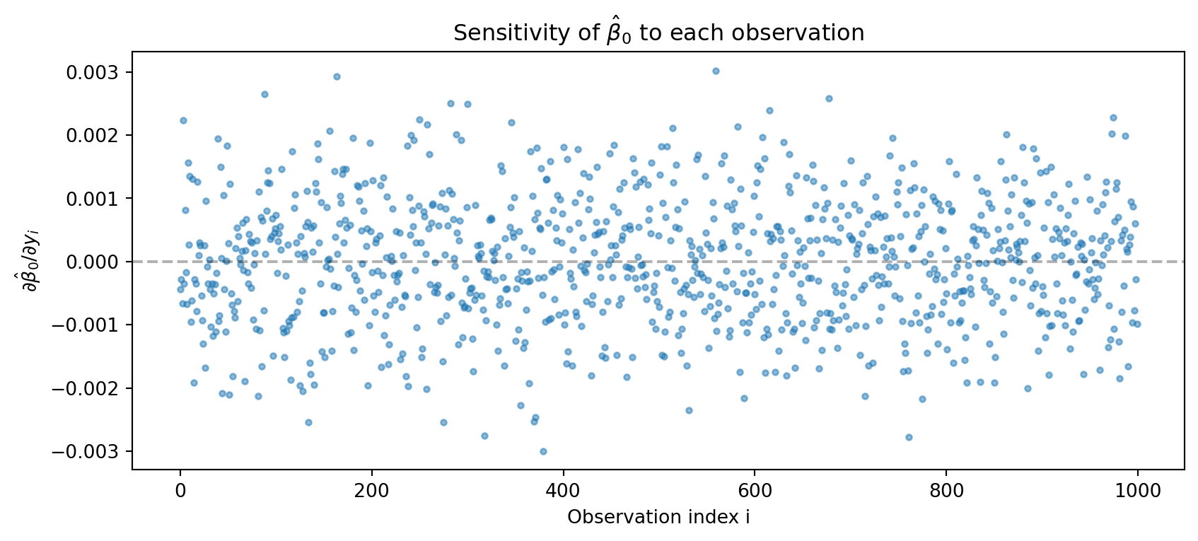
Most influential observation indices: [318 761 163 379 559]
Their sensitivities: [-0.00275735 -0.00278138  0.00292967 -0.00299568  0.00301899]
Their X values:
[[-2.851877   -0.3963519  -0.7369024 ]
 [-2.8574488   0.30645004  0.1899148 ]
 [ 3.0336585  -0.6308674   0.83326805]
 [-3.0904574   0.59396833 -0.34163857]
 [ 3.0960157  -1.7181016  -0.59638846]]
Interpretation:
The sensitivity \(\partial \hat{\beta}_0 / \partial y_i\) depends on \((Xg)_i\) where \(g = (X^\top X)^{-1} e_0\). This is essentially the \(i\)-th row of \(X\) projected onto the direction that most affects \(\hat{\beta}_0\). Observations with extreme \(X\) values in the relevant direction have higher sensitivity.
This is directly related to leverage in regression. The leverage of observation \(i\) is \(h_{ii} = X_i (X^\top X)^{-1} X_i^\top\). High-leverage points have \(X\) values far from the mean, giving them more “pull” on the regression line. Our sensitivity analysis shows exactly how much each observation affects a specific coefficient.
Question 3.6 (Extra Credit): Sensitivity to X
The full adjoint rule also gives \(\bar{X}\). Compute and interpret the sensitivity of \(\hat{\beta}_0\) to changes in \(X_{ij}\).
# modify here: compute X_bar using the full adjoint formula
# X_bar = r @ g.T - (X @ g) @ beta_hat.T
# This gives d(beta_hat[0])/d(X_ij) for all i,j
# SOLUTIONS
# Full adjoint for X
X_bar_manual = jnp.outer(r, g) - jnp.outer(X @ g, beta_hat)
print(f"Shape of X_bar: {X_bar_manual.shape}")
print(f"X_bar[0,:] (sensitivity to first row of X): {X_bar_manual[0]}")
# Verify with JAX
def lls_X(X):
return jnp.linalg.lstsq(X, y)[0]
_, vjp_fun_X = vjp(lls_X, X)
X_bar_jax, = vjp_fun_X(beta_bar)
print(f"Match: {jnp.allclose(X_bar_manual, X_bar_jax, atol=1e-5)}")
# Visualize X sensitivities
plt.figure(figsize=(12, 4))
for j in range(p):
plt.subplot(1, p, j+1)
plt.plot(X_bar_manual[:, j], 'o', alpha=0.3, markersize=2)
plt.xlabel('Observation i')
plt.ylabel(f'$\\partial \\hat{{\\beta}}_0 / \\partial X_{{i,{j}}}$')
plt.title(f'Sensitivity to column {j}')
plt.tight_layout()
plt.show()Shape of X_bar: (1000, 3)
X_bar[0,:] (sensitivity to first row of X): [ 0.00078793 -0.00044138 0.00021814]
Match: True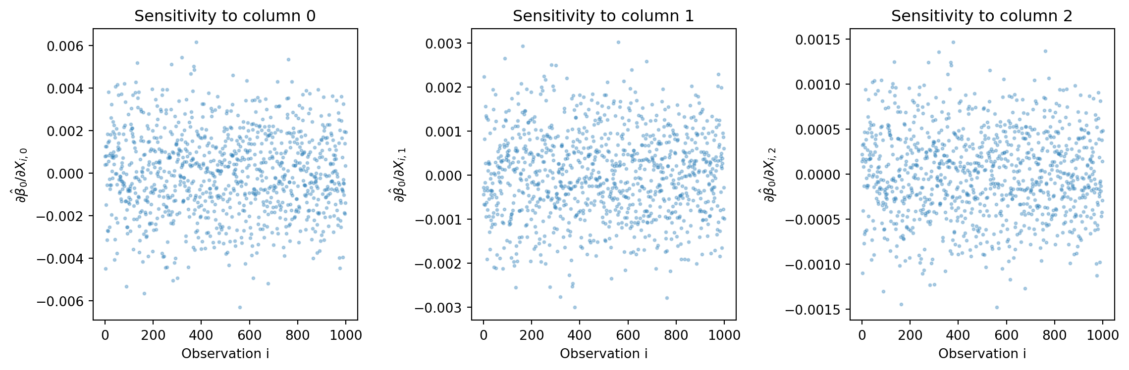
(double click to edit your answer)
What is the computational advantage of using the adjoint/VJP approach for this sensitivity analysis compared to finite differences?
Computational advantage:
Finite differences: To compute all \(n \times p\) sensitivities \(\partial \hat{\beta}_0 / \partial X_{ij}\), we would need \(n \times p\) separate LLS solves (perturbing each \(X_{ij}\) one at a time). For our problem: \(1000 \times 3 = 3000\) solves.
VJP/Adjoint: We need only one backward pass which involves:
- One linear solve: \((X^\top X)^{-1} \bar{\beta}\) - \(O(p^3)\)
- Matrix-vector products - \(O(np)\)
Total: \(O(np + p^3)\) vs \(O(np \cdot (np^2 + p^3))\) for finite differences.
For large \(n\), this is roughly \(n \times p\) times faster! This is why adjoint methods are essential for sensitivity analysis in large-scale problems.